In this tutorial we show how to calculate frequencies of molecules with MLatom. We will basically continue from geometry optimization tutorial, as it is a common practice to first optimize geometry and then calculate its frequency, i.e., to check whether it is a true minimum or transition state (number of imaginary frequencies) and obtain ZPVE and other thermochemical corrections.
We start with the same example as that in the beginning of geometry optimization tutorial. Geometry optimization is typically needed before calculating frequencies and the same method or model should be used for both.
After getting the optimized geometry (opt.xyz) as described in the tutorial on geometry optimization, you can do frequency calculations with input file/command line options freq.inp shown below (see the separate section on calculating frequencies via Python API):
freq                  # 1. requests frequency calculation
ANI-1ccx              # 2. pre-trained model, the same as that used in geometry optimization
xyzfile=opt.xyz       # 3. file with optimized geometry
Similar to geometry optimization, the user needs to provide the model or method, which can be QM, ML or their combinations. Analytical Hessian is used when it is available, otherwise semianalytical (calculated with analytical gradients) or fully numerical Hessian (calculated with only energies) can be used.
xyzfile=[file name] tells MLatom in what file it can find the geometry. The user can directly use the optimized geometry output by MLatom (file defined by optxyz keyword), or provide it in XYZ format, e.g., for this example (in Angstrom, e.g., opt.xyz) which would look like:
9

C       -1.691449880     -0.315985130      0.000000000
H       -1.334777040      0.188413060      0.873651500
H       -1.334777040      0.188413060     -0.873651500
H       -2.761449880     -0.315971940      0.000000000
C       -1.178134160     -1.767917280      0.000000000
H       -1.534806620     -2.272315330      0.873651740
H       -1.534807450     -2.272316160     -0.873650920
O        0.251865840     -1.767934180     -0.000001150
H        0.572301420     -2.672876720      0.000175020
After you created the input file, you can run MLatom, e.g., on XACS cloud, as:
mlatom freq.inp &> freq.out
The program output will be saved in file freq.out.
Alternatively, you can run the same simulation in the command line with the same options:
mlatom freq ANI-1ccx xyzfile=opt.xyz
You should be able to find in the MLatom output the vibration analysis and thermochemistry results. The vibration analysis prints out frequency, reduced mass and force constant of each normal mode. The thermochemistry part prints out zero-point energy, enthalpy, Gibbs free energy, heat of formation and other properties. For our example, the part of the output would look like:
==============================================================================
                    Vibration analysis for molecule      1
==============================================================================
Multiplicity: 1
Rotational symmetry number: 1
This is a nonlinear molecule
Mode     Frequencies     Reduced masses     Force Constants
            (cm^-1)            (AMU)           (mDyne/A)
    1        261.0407          1.0929             0.0439
    2        286.9474          1.1295             0.0548
    3        428.0328          2.7260             0.2943
    4        841.1644          1.0947             0.4564
    5        928.2688          2.3346             1.1853
    6       1082.6338          3.1779             2.1946
    7       1138.6399          1.9583             1.4959
    8       1212.5257          1.5518             1.3442
    9       1287.5002          1.1134             1.0874
    10       1292.8263          1.0682             1.0520
    11       1426.7497          1.2307             1.4760
    12       1457.4408          1.3203             1.6524
    13       1496.9454          1.1496             1.5178
    14       1501.2654          1.0458             1.3887
    15       1524.8936          1.0529             1.4426
    16       3063.7060          1.0530             5.8232
    17       3076.9020          1.1120             6.2026
    18       3093.2039          1.0342             5.8299
    19       3201.4189          1.1000             6.6424
    20       3213.8757          1.1004             6.6964
    21       3741.4822          1.0681             8.8098
==============================================================================
                    Thermochemistry for molecule      1
==============================================================================
Standard deviation of NNs                :      0.00063190 Hartree         0.39652 kcal/mol
Energy                                   :   -154.89195912 Hartree

ZPE-exclusive internal energy at      0 K:      -154.89196 Hartree
Zero-point vibrational energy            :         0.08101 Hartree
Internal energy                  at   0 K:      -154.81095 Hartree
Enthalpy                         at 298 K:      -154.80576 Hartree
Gibbs free energy                at 298 K:      -154.83631 Hartree

Atomization enthalpy             at   0 K:         1.21200 Hartree       760.54458 kcal/mol
ZPE-exclusive atomization energy at   0 K:         1.29301 Hartree       811.37653 kcal/mol
Heat of formation                at 298 K:        -0.09030 Hartree       -56.66187 kcal/mol
Choosing the method or model
The user can benefit from MLatom’s many choices of the methods or models. Many methods such as ANI-1ccx or AIQM1 are recognized automatically by MLatom as shown above. We also show examples of using QM method (B3LYP/6-31G*) and user-trained ML model (ANI model).
The general way to define the QM method is to use method and the corresponding QM program providing its implementations (MLatom uses interfaces to such programs). For example, the input file of using B3LYP/6-31G*:
freq                    # 1. requests frequency calculation
method=B3LYP/6-31G*     # 2. requests running DFT calculation with B3LYP
qmprog=PySCF            # 3. requests using PySCF for B3LYP calculations; qmprog=Gaussian can also be used
xyzfile=opt.xyz         # 4. file with optimized geometry
The general way to request the frequency calculations with the user-trained ML model is to specify the ML model type with MLmodelType and MLmodelIn keyword. For example, the input file of using ANI model:
freq                    # 1. requests frequency calculation
MLmodelType=ANI         # 2. request optimization with the ANI-type of machine learning potential
MLmodelIn=ani.npz       # 3. the file with the trained model should be provided, here it is ani.npz file
xyzfile=opt.xyz         # 4. file with optimized geometry
The advanced user-defined hybrid models such as delta-learning models can be used for frequency calculation only via Python API as demonstrated separately.
Note
In principle, our default recomendation is to use AIQM1 as it is usually the most accurate method for affordable cost. However, it is currently only applicable to the compounds with CHNO elements. Another limitation is that to unlock its full potential, we recommend to install the MNDO program for its QM part. The XACS cloud uses Sparrow instead, which currently only provides numerical gradients and Hessians severly limiting its applicability for frequency calculations. ANI-1ccx is hence a good alternative on the XACS cloud if it can be applied (it has additional limitations to neutral closed-shell compounds in ground state).
Also, currently, among ML models, Hessians are currently available only for ANI-type models.
Calculations of many molecules
MLatom can also perform frequency calculations of many molecules like geometry optimization. MLatom will output the vibration analysis and thermochemical properties of each molecule.
To do these calculations, you simply need to prepare the XYZ file with the geometries of multiple molecules (or get this file from MLatom’s previous geometry optimization calculations), e.g., for the hydrogen and methane molecules your opt.xyz file may look like:
2

1         0.0000000000        0.0000000000        0.0000000000
1         0.7414000000        0.0000000000        0.0000000000
5

C         0.0000000000        0.0000000000        0.0000000000
H         1.0870000000        0.0000000000        0.0000000000
H        -0.3623333220       -1.0248334322       -0.0000000000
H        -0.3623333220        0.5124167161       -0.8875317869
H        -0.3623333220        0.5124167161        0.8875317869
Charge and multiplicity
A quick reminder on how to define the charges and multiplicities of a single or multiple molecules. The input might looks something like:
freq                    # 1. requests frequency calculation
AIQM1                   # 2. AI-enhanced quantum mechanical method 1
xyzfile=opt.xyz         # 3. file with optimized geometries
charges=0,1             # 4. charge of the first molecule is 0, of the second is 1.
multiplicities=1,2      # 5. multiplicity of the first molecule is 1, second - 2
Note
It does not make sense to define charges and multiplicities for models like ANI-1ccx which were trained on the neutral closed-shell species.
Choosing the program
MLatom provides several ways (programs) to calculate frequencies and thermochemical properties, similarly to geometry optimizations, the user can choose the program with the keyword optprog (not freqprog). Two options are available:
optprog=Gaussian and optprog=ASE for using the respective programs.
These are actually different tasks and while they are split in Python API (see below), in input file, when freq is requested, both tasks are performed.
optprog=Gaussian will perform both tasks with Gaussian and will generate input and output files which the user can modify and inspect. Gaussian’s interface is the most time-tested and hence, robust, but not available on the XACS cloud and needs to be installed by the user locally.
If optprog=ASE is requested, the ASE is used to calculate thermochemical properties following the frequencies calculations performed either with the improved code based on TorchANI (modified to correctly capture the negative frequency in transition states) or PySCF. Frequencies given by modified TorchANI’s code was also tested by us and available on the XACS cloud. PySCF can be only choosen through Python API.
If no optprog is provided, by default, MLatom will check whether Gaussian is available and use it, otherwise it will use ASE & modified TorchANI combination.
Whatever program you chhose, it is worth checking the instructions below for pitfalls and tips.
ASE
For MLatom version older than 3.1.1, the user should tell ASE whether molecules are linear by using ase.linear keyword. If the molecule is linear, you need to set this value as 1, otherwise it is by default 0. If your input XYZ file has more than 1 molecule, ase.linear=1 makes MLatom assume that they are all linear molecules. You can specify the linearity by, e.g., ase.linear=1,0. For version newer than 3.1.1 (including), MLatom can automatically detect the linearity of molecules so you don’t have to specify explicitly. But you can still do that which will override MLatom’s judgement.
It is also important to specify the symmetry of your molecules by using keyword ase.symmetrynumber. The default one in MLatom corresponds to
Point Group |
Symmetry number |
|---|---|
For example, if your input XYZ file has hydrogen (belongs to
freq
ANI-1ccx
xyzfile=opt.xyz
optprog=ase
ase.linear=1,0
ase.symmetrynumber=2,12
Gaussian
When Gaussian is used, you will see the gaussian.log file which is similar to the common Gaussian output file with the difference, that it will use the MLatom’s model to predict Hessian to perform the frequency calculations. Then you can use your favorite tools to analyze this output as usual for Gaussian, which is a big advantage for the Gaussian users. Here is the input file of using Gaussian to calculate frequencies.
freq
ANI-1ccx
xyzfile=opt.xyz
optprog=Gaussian
For above example, you can check the MLatom’s output file:
==============================================================================
                    Vibration analysis for molecule      1
==============================================================================
Multiplicity: 1
This is a nonlinear molecule
Mode     Frequencies     Reduced masses     Force Constants
            (cm^-1)            (AMU)           (mDyne/A)
    1        264.1253          1.0872             0.0447
    2        288.7816          1.1305             0.0555
    3        429.1248          2.7295             0.2961
    4        840.9571          1.0959             0.4566
    5        929.0118          2.3254             1.1825
    6       1083.2419          3.1763             2.1960
    7       1138.7381          1.9666             1.5025
    8       1211.7614          1.5471             1.3384
    9       1291.9096          1.0694             1.0516
    10       1299.4679          1.1131             1.1074
    11       1434.7836          1.2319             1.4941
    12       1464.0813          1.3257             1.6743
    13       1497.4787          1.1427             1.5097
    14       1502.1301          1.0457             1.3902
    15       1525.4126          1.0539             1.4449
    16       3045.3746          1.0531             5.7544
    17       3061.9747          1.1130             6.1482
    18       3092.9313          1.0343             5.8295
    19       3197.6062          1.0999             6.6261
    20       3213.0380          1.1000             6.6905
    21       3741.0501          1.0681             8.8073
==============================================================================
                    Thermochemistry for molecule      1
==============================================================================
Standard deviation of NNs                :      0.00062817 Hartree         0.39419 kcal/mol
Energy                                   :   -154.89196013 Hartree

ZPE-exclusive internal energy at      0 K:      -154.89196 Hartree
Zero-point vibrational energy            :         0.08100 Hartree
Internal energy                  at   0 K:      -154.81096 Hartree
Enthalpy                         at 298 K:      -154.80578 Hartree
Gibbs free energy                at 298 K:      -154.83631 Hartree

Atomization enthalpy             at   0 K:         1.21202 Hartree       760.55134 kcal/mol
ZPE-exclusive atomization energy at   0 K:         1.29301 Hartree       811.37710 kcal/mol
Heat of formation                at 298 K:        -0.09032 Hartree       -56.67409 kcal/mol
The examples of the full MLatom and Gaussian output files can be downloaded too.
An additional important advantage is that the advanced users can modify the gaussian.com file which contains the input required for geometry optimization with MLatom’s models.
After the gaussian.com file is modified, you can run with it the Gaussian job as usual, e.g., in your system like g16 gaussian.com in command line.
Calculations through Python API
The Python API provides more flexibility to use more complicated models and build custom workflows.
Below is a workflow of optimizing geometry and calculating frequency. You might already see some of the codes in geometry optimization tutorial.
import mlatom as ml

# Get the initial guess for the molecules to optimize
initmol = ml.data.molecule.from_xyz_file('init.xyz')

# Choose one of the predifined (automatically recognized) methods
mymodel = ml.models.methods(method='ANI-1ccx')

# Optimize the geometry with the choosen optimizer:
geomopt = ml.optimize_geometry(model=mymodel, initial_molecule=initmol, program='ASE', maximum_number_of_steps=10000)

# Get the optimized molecule
final_mol = geomopt.optimized_molecule

# Do vibration analysis and thermochemistry calculation
freq = ml.thermochemistry(model=mymodel, molecule=final_mol, program='ASE')
# or vibration analysis only
# freq = ml.freq(model=mymodel, molecule=final_mol, program='')

# Save the molecule with vibration analysis and thermochemistry results
final_mol.dump(filename='final_mol.json',format='json')

# Check vibration analysis
print("Mode     Frequencies     Reduced masses     Force Constants")
print("           (cm^-1)            (AMU)           (mDyne/A)")
for ii in range(len(final_mol.frequencies)):
    print("%d   %13.4f   %13.4f   %13.4f"%(ii,final_mol.frequencies[ii],final_mol.reduced_masses[ii],final_mol.force_constants[ii]))

# Check thermochemistry results
print(f"Zero-point vibrational energy: {final_mol.ZPE} Hartree")
print(f"Enthalpy at 298 K: {final_mol.H} Hartree")
print(f"Gibbs Free energy at 298 K: {final_mol.G} Hartree")
print(f"Heat of formation at 298 K: {final_mol.DeltaHf298} Hartree")
You can compare your results with the output shown above.
Note
Note that ml.thermochemistry contains both vibration analysis and thermochemistry calculation. If you just want vibrational analysis, you can use ml.freq instead. All the results are saved as the arguments of final_mol.
There will be several properties related to thermochemistry listed below that are attributed to the molecule object (in Hartree for energies and Hartree/K for entropy) after calculation:
{...
'ZPE': 0.080996,             # Zero-point energy
'DeltaE2U': 0.085241,        # Difference between internal energy and total energy (ZPVE-exclusive)
'DeltaE2H': 0.086185,        # Difference between enthalpy and total energy (ZPVE-exclusive)
'DeltaE2G': 0.055654,        # Difference between Gibbs free energy and total energy (ZPVE-exclusive)
'U0': -154.810964,           # Internal energy at 0 K
'H0': -154.810964,           # Enthalpy at 0 K
'U:' -154.80672,             # Internal energy at 298 K
'H': -154.805775,            # Enthalpy at 298 K
'G': -154.836306,            # Gibbs free energy at 0 K
'S': 0.00010240004758876359, # entropy
'atomization_energy_0K': 1.2120157100000029,
'ZPE_exclusive_atomization_energy_0K': 1.293011710000003,
'DeltaHf298': -0.0903159176864495  # Heat of formation at 298 K
}
You can retrieve the value of the property by directly calling molecule.property (e.g. molecule.G will return you the Gibbs free energy of the molecule).
Calculations with custom hybrid models
Finally, a more advanced example of using a custom delta-learning model, trained on the differences between full configuration interaction and Hartree–Fock energies:
XYZ coordinates, full CI energies and Hartree–Fock energies of the training points can be downloaded here (xyz_h2_451.dat, E_FCI_451.dat, E_HF_451.dat). You can try to train the delta-learning model by yourself. Here, we provide a pre-trained model using ANI delta_FCI-HF_h2_ani.npz.
import mlatom as ml

# Get the initial guess for the molecules to optimize
initmol = ml.data.molecule.from_xyz_file('h2_init.xyz')

# Let's build our own delta-model
# First, define the baseline QM method, e.g.,
baseline = ml.models.model_tree_node(name='baseline', operator='predict', model=ml.models.methods(method='HF/STO-3G', program='pyscf'))
# Second, define the correcting ML model, in this case the ANI model trained on the differences between full CI and HF
delta_correction = ml.models.model_tree_node(name='delta_correction', operator='predict', model=ml.models.ani(model_file='delta_FCI-HF_h2_ani.npz'))
# Third, build the delta-model which would sum up the predictions by the baseline (HF) with the correction from ML
delta_model = ml.models.model_tree_node(name='delta_model', children=[baseline, delta_correction], operator='sum')

# Optimize the geometry with the delta-model as usual:
geomopt = ml.optimize_geometry(model=delta_model, initial_molecule=initmol, program='ASE')

# Get the final geometry approximately at the full CI level
final_mol = geomopt.optimized_molecule
print('Optimized coordinates:')
print(final_mol.get_xyz_string())
final_mol.write_file_with_xyz_coordinates(filename='final.xyz')

# Let's check how many full CI calculations, our delta-model saved us
print('Number of optimization steps:', len(geomopt.optimization_trajectory.steps))

# Calculate frequency
freq = ml.freq(model=delta_model, molecule=final_mol, program='')

# Check vibration analysis
print("Mode     Frequencies     Reduced masses     Force Constants")
print("           (cm^-1)            (AMU)           (mDyne/A)")
for ii in range(len(final_mol.frequencies)):
    print("%d   %13.4f   %13.4f   %13.4f"%(ii,final_mol.frequencies[ii],final_mol.reduced_masses[ii],final_mol.force_constants[ii]))
Given an initial geometry h2_init.xyz, you will get the following output when using the codes above.
Optimized coordinates:
2

H             0.1272159900000           0.0000000000000           0.0000000000000
H             0.8727840100000           0.0000000000000           0.0000000000000

Number of optimization steps: 7
Mode     Frequencies     Reduced masses     Force Constants
        (cm^-1)            (AMU)           (mDyne/A)
0       4327.2885          1.0078         11.1190
Thermochemistry in Diels–Alder reaction
By using these thermochemical properties, you can easily evaluate relative energies for various aspects of chemical behavior,
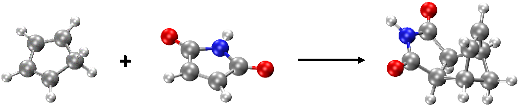
such as the change of energy profile during reaction process. We take the Diels–Alder reaction of cyclopentadiene and maleimide, an example in the MLatom 3 paper. You can download the geometry file needed here: re.xyz.
There are 3 structures in re.xyz: the first two strucutres are reactants and the third one is the product (see figure below):
Thus, the basic idea here is that we will calculate thermochemical properties for each molecule and then calculate the energy changes from product to reactants. We will illustrate that it is very convenient to do with the Python API (the same can be done manually through input file/command line calculations by performing thermochemical calculations for each molecule and get the changes in each type of energy).
import mlatom as ml

# read molecules from .xyz file
reDB = ml.data.molecular_database().read_from_xyz_file('re.xyz')
optreDB = ml.data.molecular_database()

# define method to calculate thermochemical properties
model = ml.models.methods(method='AIQM1', qm_program='mndo')

for mol in reDB:

    # geometry optimization
    geomopt = ml.optimize_geometry(model=model, initial_molecule=mol, program='gaussian')
    optmol = geomopt.optimized_molecule

    # frequency calculation
    ml.thermochemistry(model=model, molecule=optmol)
    optreDB.append(optmol)

# get relative energies
deltaE = optreDB[2].energy - optreDB[1].energy - optreDB[0].energy
deltaG = optreDB[2].G - optreDB[1].G - optreDB[0].G
deltaH = optreDB[2].H - optreDB[1].H - optreDB[0].H
print(deltaE)
print(deltaG)
print(deltaH)
Here is the summary of the output containing changes in ZPVE-exclusive energy, Gibbs free energy, and enthalpy.
Method |
|||
|---|---|---|---|
reference |
-34.20 |
- |
- |
AIQM1 |
-34.13 |
-15.98 |
-30.36 |
This shows that if you can use AIQM1, you should use this method to obtain accurate results fast; it is often much more preferable than performing analogous, slower and less accurate, DFT calculations.
Any questions or suggestions?
If you have further questions, criticism, and suggestions, we would be happy to receive them in English or Chinese via email, Slack (preferred), or WeChat (please send an email to request to add you to the XACS user support group).