Single-point calculations with QM methods

MLatom supports single-point QM calculations with various popular programs such as Gaussian, PySCF, xTB, etc. Detailed manuals for simulations with QM methods can be found in Simulations with QM methods.

The typical input file for single-point calculations should contain xyzfile which defines geometry file and yestfile which defines the file to store energy. For QM methods, users need to provide the method name and qmprog, i.e. the corresponding QM program. Here is an example of the input file for energy-only calculations at B3LYP/6-31G* level with Gaussian

method=B3LYP/6-31G*
qmprog=gaussian
xyzfile=sugar_iso.xyz
yestfile=enest.dat

By running the command $mlatom mlatom.inp > mlatom.out, you will the get the MLatom output file as follows:

******************************************************************************

Energy of molecule      1:        -687.1484077000000 Hartree
Energy of molecule      2:        -687.1383648000000 Hartree

==============================================================================
Wall-clock time: 83.08 s (1.38 min, 0.02 hours)

MLatom terminated on 03.02.2024 at 09:35:57
==============================================================================

In the output file, energies of two molecules are listed in the same order as that in the input .xyz file.

Single-point calculations with hybrid QM/ML methods

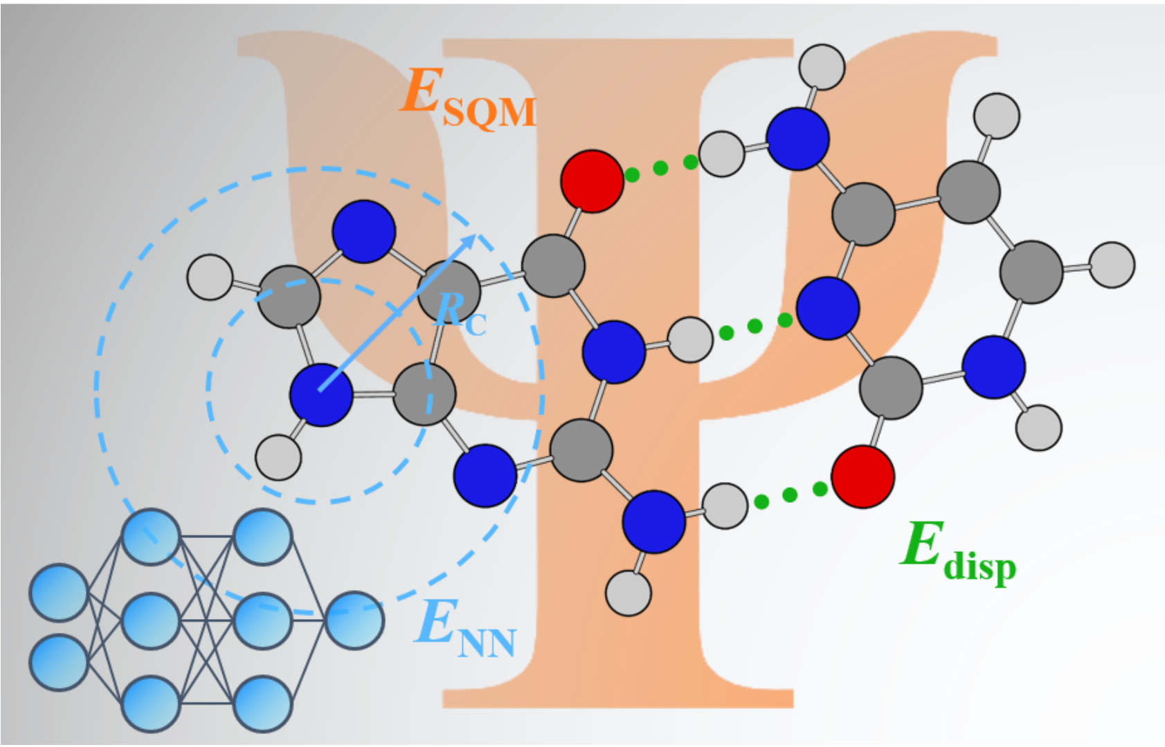
One of the successful examples of hybrid QM/ML method is AIQM1, which is a general-purpose method approaching the gold-standard coupled cluster QM method at the cost of low-level semiempirical QM method. It takes the advantage of delta-learning strategy, correcting less accurate semiempirical method with state-of-art ML model ensemble (see figure below). Beyond this, in MLatom, users can also define their own delta-learning model, which is currently easy to achieve with Python API (see python API tutorial).

For AIQM1, users just need to request AIQM1 calculation in the first line:

AIQM1                     # 1. request AIQM1 method
xyzfile=sugar_iso.xyz     # 2. file with geometry
yestfile=enest.dat        # 3. file to store energy

After running the command $mlatom mlatom.inp > mlatom.out, users will get the mlatom.out as :

******************************************************************************

Properties of molecule 1

Standard deviation of NN contribution    :      0.00094895 Hartree         0.59548 kcal/mol
NN contribution                          :      0.00275644 Hartree
Sum of atomic self energies              :   -578.89384843 Hartree
ODM2* contribution                       :   -107.70671483 Hartree
D4 contribution                          :     -0.00358197 Hartree
Total energy                             :   -686.60138879 Hartree


Properties of molecule 2

Standard deviation of NN contribution    :      0.00066560 Hartree         0.41767 kcal/mol
NN contribution                          :      0.00159327 Hartree
Sum of atomic self energies              :   -578.89384843 Hartree
ODM2* contribution                       :   -107.68954498 Hartree
D4 contribution                          :     -0.00351388 Hartree
Total energy                             :   -686.58531402 Hartree

==============================================================================
Wall-clock time: 0.77 s (0.01 min, 0.00 hours)

MLatom terminated on 03.02.2024 at 09:20:02
==============================================================================

For each molecule, all the energy components contained in AIQM1 method are presented, including ODM2* energy, D4 enengy and NN energy (sum of NN contribution and atomic self energies), The standard deviation of NN contribution can be used to judge whether AIQM1 is reliable.

As a comparison, we show here isomeration energies calculated by each method and their respective times used.

Single-point calculations with user-trained ML models

MLatom can read a user-trained model from a file and make predictions with it for new data (given either as input vectors X or as XYZ coordinates). Users should provide either MLmodelType and/or MLprog argument. Below is the table for type of ML models and programs available:

We will use a pretrained MACE model to predict molecular enenrgy. You can download mace model file here: mace.pt. Here is an example of how to use user-trained MACE model to perform single-point calculation:

useMLmodel              # 1. requests usage of ML model for prediction
MLmodelType=MACE         # 2. request the MACE model
MLmodelIn=mace.pt       # 3. the file with the trained model should be provided, here it is mace.pt file
xyzfile=sugar_iso.xyz   # 4. file with geometries

For how to train ML models with MLatom, please refer to manual.

Gradients and Hessian

If users need gradients and Hessian, two lines can be added in the input file:

AIQM1                       # 1. request AIQM1 method
xyzfile=sugar_iso.xyz       # 2. file with geometry
yestfile=enest.dat          # 3. file to store energy
ygradxyzestfile=grad.dat    # 4. file to store gradients
hessianestfile=hess.dat     # 5. file to store hessian

ygradxyzestfile will create the file storing the gradients and hessianestfile the Hessian. These keywords are case-insensitive but the file names are.

Charge and multiplicity

If molecules have other than default charges (default 0) and multiplicities (default 1), the input might look like:

method=B3LYP/6-31G*
qmprog=gaussian
xyzfile=sp.xyz
yestfile=enest.dat
charges=0,1
multiplicities=1,3

Calculations through PyAPI

method = mlatom.models.methods(method='b3lyp/6-31G*', program='gaussian')
# method = mlatom.models.methods(method='b3lyp/6-31G*', program='pyscf', nthreads=18)

import mlatom as ml
# read molecule from .xyz file
molDB = ml.data.molecular_database.from_xyz_file('sugar_iso.xyz')

# define method
model = ml.models.methods(method='AIQM1')
# model = ml.models.methods(method='B3LYP/6-31G*'. program='pyscf')  ## calculations using QM methods

model.predict(molecular_database=molDB)

print(molDB[0].energy)
print(molDB[1].energy)
print(molDB[1].energy-molDB[0].energy)

model.predict(molecular_database=mol, calculate_energy_gradients=True, calculate_hessian=True)

mol = ml.data.molecule.from_xyz_file('sp.xyz')

model.predict(molecule=mol)

mol.charge = 1
mol.multiplicity = 3

molDB.charges = [1,1]
molDB.multiplicities = [1,3]

mol.energy
mol.get_energy_gradients()
mol.hessian

molDB.get_properties('energy')
molDB.get_xyz_vectorial_properties('energy_gradients')
molDB.get_properties('hessian')

baseline=ml.models.model_tree_node(name='baseline', operator='predict', model=ml.models.methods(method='HF/STO-3G', program='pyscf')
delta_correction=ml.models.model_tree_node(name='delta_correction', operator='predict', model=ml.models.ani(model_file='delta_FCI-HF_h2_ani.npz')`

ml.models.model_tree_node(name='hybrid', operator='sum', children=[baseline, delta_correction])

import mlatom as ml

# Get the initial guess for the molecules to optimize
mol = ml.data.molecule.from_xyz_file('h2_init.xyz')

# Let's build our own delta-model
# First, define the baseline QM method, e.g.,
baseline = ml.models.model_tree_node(name='baseline', operator='predict', model=ml.models.methods(method='HF/STO-3G', program='pyscf'))
# Second, define the correcting ML model, in this case the KREG model trained on the differences between full CI and HF
delta_correction = ml.models.model_tree_node(name='delta_correction', operator='predict', model=ml.models.ani(model_file='delta_FCI-HF_h2_ani.npz'))
# Third, build the delta-model which would sum up the predictions by the baseline (HF) with the correction from ML
delta_model = ml.models.model_tree_node(name='delta_model', children=[baseline, delta_correction], operator='sum')

delta_model.predict(molecule=mol)

print(mol.energy)