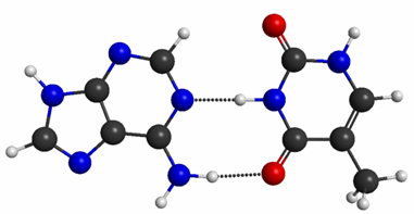
Prof. Peifeng Su's group has recently developed the GKS-EDA(TD) method, which is based on GKS-EDA, for quantitatively investigating the nature of intermolecular interactions in excited states. We demonstrate the capabilities of GKS-EDA(TD) by using the intermolecular interactions of the first excited state of the AT base pair (abbreviated as AT(WC)) as an example.

Below is an example of a GKS-EDA(TD) input file for studying the first excited state of the AT(WC) base pair at the LC-PBE/6-31++G** level.

The transition from the ground state to the first excited state (S0→S1) of AT(WC) is primarily an n→π* transition on base T. To edit the input file, place the atomic coordinates of the excited monomer in the front and those of base A in the back, as shown below. Edatyp=tdeda inside $lmoeda designates to carry out the GKS-EDA(TD). The keywords 'irtfrg' and 'irtsup' are used to refer to excited states, specifically the excited state of the monomer and the excited state of the supramolecule, respectively. When 'irtfrg' is equal to 1, it indicates the first excited state of the monomer. Similarly, 'irtsup' has the same significance. 'tdtol' refers to the truncation coefficient of the determinant of the excited state, which is typically set to 0.01 to balance computational efficiency and accuracy. MATOM, MCHARG, and MMULT refer to the number of atoms, charge, and multiplicity contained in the recognized monomer, respectively.

If the parameters $TDDFT and TDDFT=excite edatyp=tdeda irtsup=1 irtfrg=1 tdtol=0.01 are removed, the system will automatically perform the calculation in the ground state.

$contrl runtyp=eda TDDFT=excite DFTTYP=pbe $end
 $contrl icharg=0 mult=1 maxit=200
ISPHER=1 $end
 $TDDFT TAMMD=.F. nstate=20 $end
 $lmoeda edatyp=tdeda irtsup=1
irtfrg=1 tdtol=0.01
  MATOM(1)=15 15 MCHARG(1)=0 0 MMULT(1)=1
1 $end
 $basis gbasis=n31 ngauss=6 ndfunc=1
diffsp=.t. npfunc=1 diffs =.t. $end
 $scf diis=.t. soscf=.f. dirscf=.t.
fdiff=.f. $end
 $dft nrad=99 nthe=36 nphi=72 lc=.t.
$end
 $system mwords=1000 $end
 $data
 AT
 c1
C     6.0     2.48806810    -0.82872897     0.00010200
C     6.0     3.94698000    -0.80676401    -0.00004200
N     7.0     1.85999000     0.40153500     0.00018400
O     8.0     1.82807899    -1.87023199     0.00014700
C     6.0     4.67908096    -2.10824394    -0.00013100
C     6.0     4.55179882     0.40222600    -0.00013700
C     6.0     2.46153092     1.63559997     0.00018100
H     1.0     0.80990797     0.40439400     0.00022700
H     1.0     4.41258621    -2.70590091     0.87867999
H     1.0     4.41239977    -2.70588493    -0.87889600
H     1.0     5.76232576    -1.95136797    -0.00024600
N     7.0     3.84490800     1.57574499    -0.00006000
H     1.0     5.63251781     0.51046699    -0.00029300
O     8.0     1.85439503     2.69294190     0.00006100
H     1.0     4.31586409     2.46916294    -0.00016600
C     6.0    -3.09782195    -0.60598898    -0.00003600
C     6.0    -3.59627700     0.69642299    -0.00010400
C     6.0    -1.69310296    -0.73755199     0.00010200
N     7.0    -4.95784807     0.53968900    -0.00017600
N     7.0    -2.89110303     1.83337796    -0.00004500
N     7.0    -4.11530018    -1.53513706    -0.00015000
N     7.0    -1.06866205    -1.91934097     0.00017600
N     7.0    -0.96649998     0.39787400     0.00015300
C     6.0    -5.20512581    -0.81166703    -0.00025900
H     1.0    -5.63619518     1.28717196    -0.00020100
C     6.0    -1.58625495     1.58854496     0.00008300
H     1.0    -0.04652500    -1.97087204     0.00022400
H     1.0    -1.61883795    -2.76393890     0.00009800
H     1.0    -6.21389914    -1.20432401    -0.00035100
H     1.0    -0.92159200     2.45012593     0.00013400
 $end

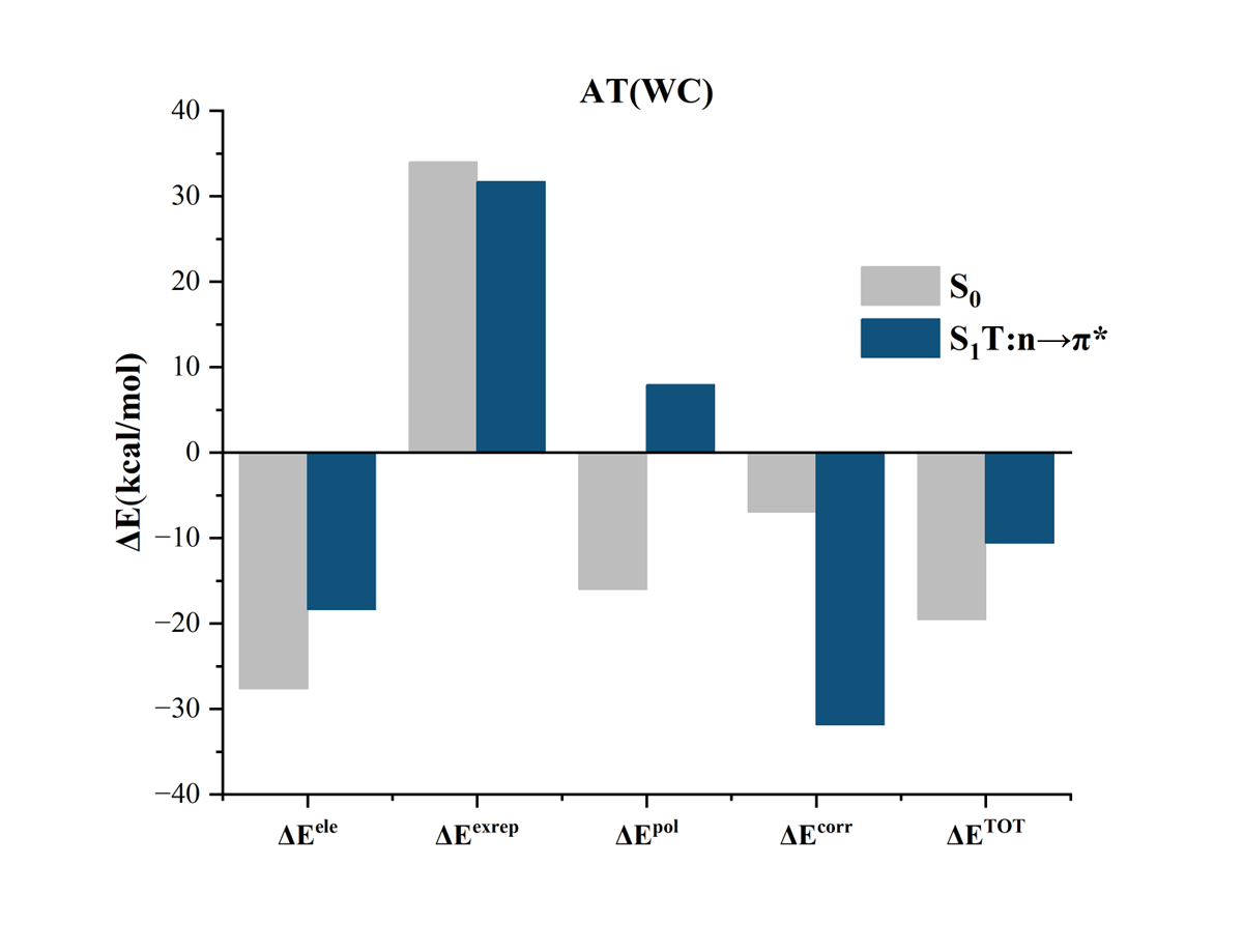
The results of the ground state and excited state EDA calculations are plotted below. It is evident that the ground state and excited state interactions differ significantly in nature. For more information, refer to the Generalized Kohn-Sham Energy Decomposition Analysis Method Based on Contained-Time DensityFunctional Theory.

NOTE: XEDA has two versions: XEDA 1.0 is developed based on GAMESS, while XEDA 2.0 is a lately developed stand-alone software. Currently, only XEDA 1.0 supports the GKS-EDA(TD) method. The XACS platform automatically recognizes the different XEDA versions, so the user does not need to specify them.

If calculating the interaction of π...π* excited states of AT(WC), please ensure the input file is set up correctly. You can check out the XEDA tutorial for more information.