6. Spectroscopy

This tutorial will use MLatom@XACS program. See its manual and tutorials for more details.

Here we will show how to use MLatom for different spectroscopic simulations:

infrared spectra
one-photon absorption (UV/vis) spectra
two-photon absorption spectra

6.1. Infrared spectra

In this example, we generate infrared (IR) spectrum of ethanol from an existing MD trajectory propagated with AIQM1 for 3 ps. See previous section on how to run dynamics. AIQM1 also generates dipole moments which are needed to calculate intensities in infrared spectra.

6.1.1. Input file

MLatom input is very simple:

IRSS                            # Infrared Spectra Simulation
TrajH5MDIn=traj.h5              # H5MD file

where the file traj.h5 is pre-acquired trajectory file with information of dipole moments inside.

6.1.2. Computational results

You can see the spectrum (ir.png) in your folder after the computation is finished:

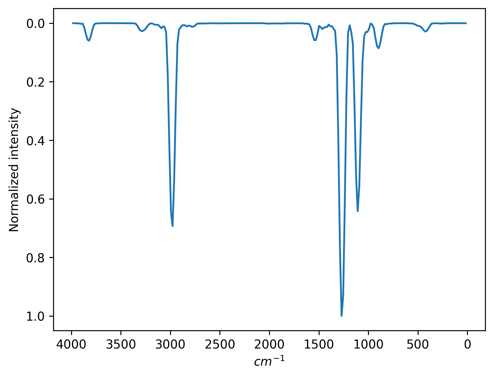
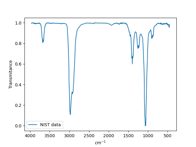
Below, for comparison, is the spectrum from the NIST database:

6.2. UV/vis absorption spectra with machine learning

Machine learning can be used to greatly accelerate the calculation of precise UV/vis absorption spectra via nuclear ensemble approach (NEA) which typically requires many hundreds or thousands of expensive quantum mechanical calculations of excited states. MLatom supports such ML-accelerated NEA calculations as described in our paper.

The following example is from our book chapter.

6.2.1. Input files

MLatom input file:

cross-section
Nexcitations=30
plotQCNEA
plotQCSPC
deltaQCNEA=0.05

These calculations require many data files (reference excitation energies at TDDFT level). These data files are zipped and should be uploaded as a zip archive to the cloud computing as auxiliary file.

6.2.2. Computational results

Calculations can take more than 5 min. MLatom automatically determines the minimum required number of training points, in this case it needed 200 points for precise spectrum. In the output file you can find that it took 4 iterations to converge:

==========================================================================================
run ML-NEA iteratively for spectrum generation ( ML_train_iter ) started at Wed Dec  1 12:00:19 2021 CST
ML-NEA iteration 1: train_number = 50; RMSE_geom = 0.06717941145022376; rRMSE = 1.0

ML-NEA iteration 2: train_number = 100; RMSE_geom = 0.09043318436728051; rRMSE = 0.25713761026721255

ML-NEA iteration 3: train_number = 150; RMSE_geom = 0.06411060145373663; rRMSE = 0.410580813729204

ML-NEA iteration 4: train_number = 200; RMSE_geom = 0.0695737045717655; rRMSE = 0.07852252732055763

ML-NEA iteration ended after 4 iteration!
run ML-NEA iteratively for spectrum generation ( ML_train_iter ) finished at Wed Dec  1 12:08:01 2021 CST |||| total spent 462.02 sec
==========================================================================================

After the calculations finished, the spectra are plotted to plot.png file in the cross-section sub-directory. It should look like:

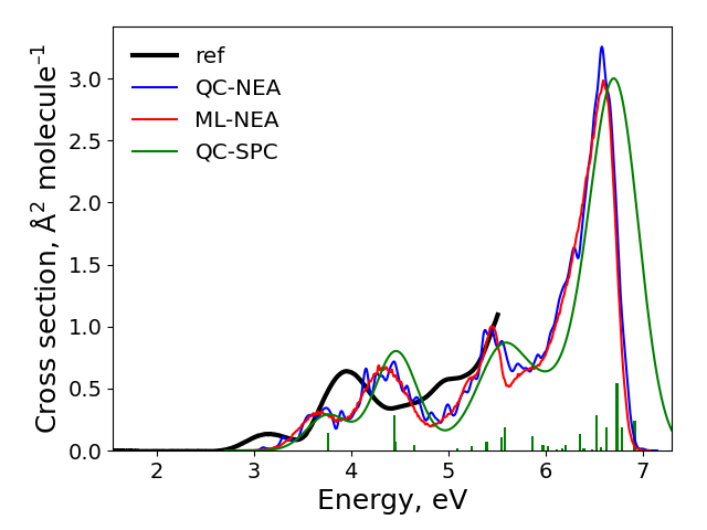
The final result: ‘ref’ is the experimental spectrum, QC-NEA – spectrum calculated with quantum chemical approach on 200 points in ensemble, ML-NEA – machine learning spectrum generated with 200 points in the training set and 50k points in ensemble, QC-SPC – spectrum generated with single-point convolution.

6.2.3. Questions

Compare obtained spectra and answer the following questions:

What are the problems with the QC-NEA spectrum?
What are the problems with the QC-SPC spectrum?
How to improve accuracy of the ML-NEA spectrum?

6.3. Two-photon absorption cross sections with machine learning

Two-photon absorption (TPA) is an important physical phenomenon which can be exploited in many different applications like upconverted laser. MLatom implements machine learning method predicting TPA cross section for a new molecule just by providing its SMILES (see this paper in Adv. Sci. for details).

6.3.1. Input files

Here we show how to calculate TPA cross section for RHODAMINE 6G and RHODAMINE 123 molecules with MLatom input file mltpa.inp:

MLTPA
SMILESfile=Smiles.csv
auxfile=_aux.txt

This input requires Smiles.csv file with SMILES of molecules:

CCNC1=CC2=C(C=C1C)C(=C3C=C(C(=[NH+]CC)C=C3O2)C)C4=CC=CC=C4C(=O)OCC.[Cl-]
COC(=O)C1=CC=CC=C1C2=C3C=CC(=N)C=C3OC4=C2C=CC(=C4)N.Cl

and optional _aux.txt, which defines the wavelength_lowbound, wavelength_upbound, and Et30 for making predicitons:

600,850,55.4
600,600,33.9

After you prepared your input files mltpa.inp, Smiles.csv, and _aux.txt, you can run MLatom as usual.

6.3.2. Computational results

After the calculations finish, the predicted TPA cross section values are saved in two files for two molecules: tpa1.txt and tpa2.txt. For our examples, they look like:

wavelength,predicted_sigma (GM)
0,285.19455
0,297.71707
0,284.11694
......
0,121.51988
0,116.537994
0,118.04909
0,103.65925
0,113.72374

and

wavelength,predicted_sigma (GM)
600.0,138.2346