1. Getting started
Here we demonstrate the capabilities of XACS platform for building a seamless user-customized computational workflow from setting up your system to calculations to the analysis of calculations and getting insights.
All exercises can be done online on XACS cloud computing without downloading and installing any of the software packages. Please register and sign (see links in the right corner of the website) and then go to Computing page to perform simulations. After you prepare input files and click on submit button, you can track the progress of the calculations in ‘My computing’ and download the output files.
To get started, our first example and exercises are for calculations and analysis of chemical bonding in a simple ethane C2H6 molecule, which consists of the following steps:
1.1. Geometry optimization of C2H6
The first step is to get the equilibrium geometry. For this, we can use many different machine learning and quantum mechanical methods and their combinations which is implemented in MLatom using interfaces to many state-of-the-art programs. A brief overview:
universal, pre-trained machine learning potentials (no need for training): ANI-1ccx (recommended), ANI-1x, ANI-2x, ANI-1x-D4, ANI-2x-D4.
hybrid quantum mechanical/machine learning methods: AIQM1 (recommended), AIQM1@DFT, and AIQM1@DFT*.
your own machine learning potential models (you can train them with MLatom) as described in the manual.
ab initio quantum mechanical methods: HF, MP2, CCSD, CASSCF, etc. (require keyword
qmprog=pyscfin input file)DFT methods, e.g.: B3LYP/6-31G*, wB97X, etc. (require keyword
qmprog=pyscfin input file)fast but approximate semi-empirical quantum mechanical methods: GFN2-xTB (does not require keyword
qmprog=), ODM2, PM6, DFTB3, AM1, MNDO, RM1, etc. (all of them require keywordqmprog=Sparrowin input file)
In this tutorial, we will try representative methods such as our own general-purpose artificial intelligence-enhanced quantum mechanical method 1 (AIQM1), pure machine learning method ANI-1ccx, and popular GFN2-xTB and B3LYP/6-31G*. Both methods are orders of magnitude faster than common DFT methods such as B3LYP/6-31G* and are more accurate as they approaches coupled-cluster accuracy for ground-state properties of neutral organic molecules. AIQM1 is more transferable than ANI-1ccx and can be applied to charged species, excited states, etc. Thus, AIQM1 is a unique method which can be used for fast and accurate geometry optimizations.
1.1.1. Input files
The input file for geometry optimization with machine-learning methods such as AIQM1 or ANI-1ccx is very simple and follows this structure:
ANI-1ccx # or AIQM1 or other machine learning-based method
geomopt
xyzfile=C2H6_init.xyz
optxyz=C2H6_opt.xyz
File C2H6_init.xyz with the initial geometry of C2H6 should be uploaded as an auxiliary file:
8

C             0.0000000000000           0.0000000000000           0.7608350816719
H            -0.0000000000000           1.0182031026887           1.1438748775511
H             0.8817897531403          -0.5091015513443           1.1438748775511
H            -0.8817897531403          -0.5091015513443           1.1438748775511
C            -0.0000000000000          -0.0000000000000          -0.7608350816719
H            -0.8817897531403           0.5091015513443          -1.1438748775511
H             0.8817897531403           0.5091015513443          -1.1438748775511
H            -0.0000000000000          -1.0182031026887          -1.1438748775511
Submit jobs with several methods: AIQM1 and ANI-1ccx.
For semi-empirical QM, ab initio and DFT methods, the input is slightly different, here we need to explicitly tell MLatom the method name with keyword method= and which QM program to use in the back-end. For example, calculations with the semi-empirical AM1 method can be performed with the interface to Sparrow using the following input file:
method=AM1
qmprog=Sparrow
geomopt
xyzfile=C2H6_init.xyz
optxyz=C2H6_opt.xyz
As another example, calculations with B3LYP/6-31G* can be performed with the interface to PySCF using the following input file:
method=B3LYP/6-31G*
qmprog=pyscf
geomopt
xyzfile=C2H6_init.xyz
optxyz=C2H6_opt.xyz
1.1.2. Computational results
After the calculations with the above input and auxiliary files are finished, you should obtain the output file with the .log extension. The output varies with the method choosen. The output of ANI-1ccx calculations should containn the lines:
  Iteration         Energy (Hartree)
           1            -79.7247066101649
           2            -79.7247066101649
           3            -79.7247651776358
           4            -79.7247966147530
           5            -79.7248710323066
           6            -79.7248832838043
           7            -79.7248873913452


Final properties of molecule 1

Standard deviation of NNs                :      0.00049813 Hartree         0.31258 kcal/mol
Energy                                   :    -79.72488739 Hartree
In the folder containing computational results, you can also find a file C2H6_opt.xyz containing the XYZ coordinates of the optimized geometry:
8

C             0.0000000000000           0.0000000100000           0.7620840000000
H             0.0000000000000           1.0168937800000           1.1584307200000
H             0.8806558500000          -0.5084468900000           1.1584307200000
H            -0.8806558500000          -0.5084468900000           1.1584307200000
C            -0.0000000000000          -0.0000000100000          -0.7620840000000
H            -0.8806558500000           0.5084468900000          -1.1584307200000
H             0.8806558500000           0.5084468900000          -1.1584307200000
H             0.0000000000000          -1.0168937800000          -1.1584307200000
The optimized geometry is shown in the following figure.

Optimized geometry of C2H6
1.1.3. Questions
Answer in WeChat the following questions.
What is the bond lengths C–C and C–H in ethane and computational time at
AIQM1,
ANI-1ccx,
AM1,
B3LYP/3-21G?
Which method would you then recommend for this molecule?
Note
You can compare the results to the experimentally known C–C bond length of 1.535 Å and C–H bond length of 1.094 Å. Be aware that rigorous statistical analysis requires comparison on many structures. Also, computational time for various methods scales very differently with the system size and the results for such a small system as ethane are not indicative.
1.2. Vibrational analysis and thermochemical calculations of C2H6
To ensure the optimized geometry is a minimum rather than a saddle point, we need to do vibrational analysis. It is usually more computatinally expensive than geometry optimization. Here we will use the geometry of C2H6 optimized before with ANI-1ccx. The calculations will also furnish lots of thermochemical properties.
1.2.1. Input file
We need to provide to MLatom very simple input file with keywords defining method ANI-1ccx, the XYZ file C2H6_opt.xyz with the optimized geometry, and requesting the frequency calculations:
ANI-1ccx
freq
xyzfile=C2H6_opt.xyz
1.2.2. Computational result
After the job is submitted and done, we can find in the output file the information about calculated frequencies as shown below:
==============================================================================
                    Vibration analysis for molecule      1
==============================================================================
Multiplicity: 1
Rotational symmetry number: 1
This is a nonlinear molecule
Mode     Frequencies     Reduced masses     Force Constants
            (cm^-1)            (AMU)           (mDyne/A)
    1        301.8021          1.0078             0.0541
    2        846.0586          1.0571             0.4458
    3        846.0587          1.0571             0.4458
    4       1015.7401          3.2294             1.9631
    5       1224.3472          1.4553             1.2853
    6       1224.3472          1.4553             1.2853
    7       1449.8617          1.2003             1.4867
    8       1501.6694          1.2591             1.6729
    9       1515.6879          1.0272             1.3903
    10       1515.6879          1.0272             1.3903
    11       1520.7107          1.0626             1.4478
    12       1520.7107          1.0626             1.4478
    13       3102.4616          1.0374             5.8831
    14       3126.4759          1.0326             5.9467
    15       3201.3230          1.0983             6.6315
    16       3201.3231          1.0983             6.6315
    17       3209.2375          1.1028             6.6922
    18       3209.2376          1.1028             6.6922
The first vibrational mode animation is shown in figure.
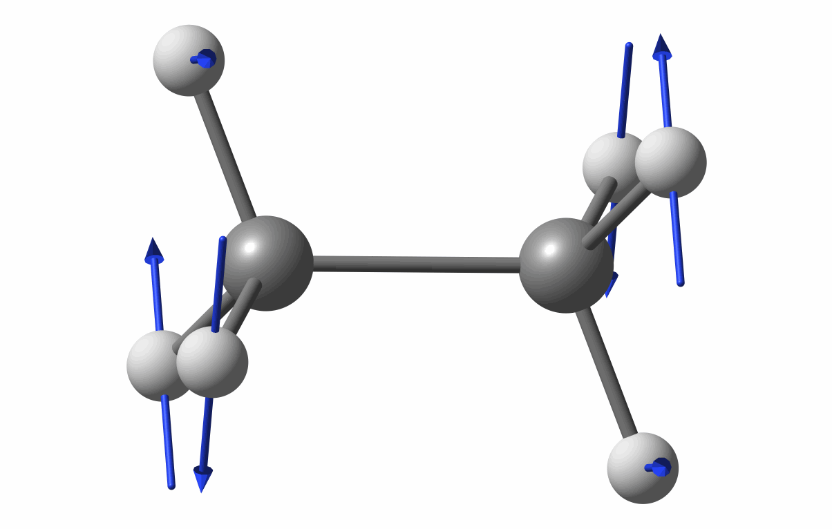
Optimized geometry of C2H6
In addition, calculations will furnish lots of additional thermochemical information such as heats of formation:
==============================================================================
                    Thermochemistry for molecule      1
==============================================================================
Standard deviation of NNs                :      0.00049813 Hartree         0.31258 kcal/mol
Energy                                   :    -79.72488739 Hartree

ZPE-exclusive internal energy at      0 K:       -79.72489 Hartree
Zero-point vibrational energy            :         0.07639 Hartree
Internal energy                  at   0 K:       -79.64849 Hartree
Enthalpy                         at 298 K:       -79.64407 Hartree
Gibbs free energy                at 298 K:       -79.67161 Hartree

Atomization enthalpy             at   0 K:         1.05923 Hartree       664.67556 kcal/mol
ZPE-exclusive atomization energy at   0 K:         1.13562 Hartree       712.61302 kcal/mol
Heat of formation                at 298 K:        -0.03085 Hartree       -19.35809 kcal/mol
1.2.3. Questions
Answer the following questions in WeChat:
Is the optimized geometry a true minimum?
What is the heat of formation of ethane at ANI-1ccx?
Note
You can compare the results to the experimentally known heat of formation at 298 K of ethane equal to −20 kcal/mol. In addition, if the neural network standard deviation is larger than 1.68 kcal/mol, the output will contain the warning that the ANI-1ccx calculations are uncertain. For AIQM1, uncertain simulations are flagged for deviations larger than 0.41 kcal/mol. See this publications on thermochemical calculations with ANI-1ccx and AIQM1.
1.3. Energy decomposition analysis of C–C bond in C2H6
After we get the equilibrium geometries optimized by ANI-1ccx, we can use the GKS-EDA method implemented in the XEDA program to have a quantitative analysis of molecular interactions for the C–C \(\sigma\)bond at the B3LYP/6-31G* level.
1.3.1. Input file
$CTR
METHOD=RHF BASIS=6-31G*
NMUL=1 CHARGE=0
DFT=B3LYP
$END
$GEO
C             0.0000000000000           0.0000000100000           0.7620840000000
H             0.0000000000000           1.0168937800000           1.1584307200000
H             0.8806558500000          -0.5084468900000           1.1584307200000
H            -0.8806558500000          -0.5084468900000           1.1584307200000
C            -0.0000000000000          -0.0000000100000          -0.7620840000000
H            -0.8806558500000           0.5084468900000          -1.1584307200000
H             0.8806558500000           0.5084468900000          -1.1584307200000
H             0.0000000000000          -1.0168937800000          -1.1584307200000
$END
$EDA
NMOL = 2
MATOM = 4 4
MMULT = 2 -2
MCHARGE = 0 0
$END
1.3.2. Computational result
After the job is finished, you can see the total interaction energy and different energy components in the output file with extension name .log (or .log.txt for cloud computation):
--------------------------------------------------------------------------------
ALL BASIS SET                                       HARTREE          KCAL/MOL
--------------------------------------------------------------------------------
ELECTROSTATIC ENERGY                  ES=          -0.223223         -140.07
EXCHANGE ENERGY                       EX=          -0.315200         -197.79
REPULSION ENERGY                     REP=           0.651096          408.57
POLARIZATION ENERGY                  POL=          -0.252414         -158.39
ELECTRON CORRELATION                CORR=          -0.039672          -24.89
GRIMME DISP CORRECTION                DC=           0.000000            0.00
TOTAL INTERACTION ENERGY               E=          -0.179414         -112.58
--------------------------------------------------------------------------------
1.3.3. Question
Based on the information provided in the output file (compare which terms are the largest), answer, what character (covalent, ionic, charge-shift, etc.) has the C–C bond.
1.4. Analysis of C–C bond in C2H6 with valence bond theory
We can perform VBSCF calculation with the XMVB program to understand the chemical bonding of the C–C \(\sigma\) bond in ethane (C2H6) molecule. Here the calculation is performed at the VBSCF/cc-pVDZ level. Two active orbitals describing the C–C \(\sigma\) bond are included in the VBSCF calculations. The VBSCF wave function includes all the structures to describe the C–C \(\sigma\) bond, and hybrid atomic orbitals (HAOs) are used.
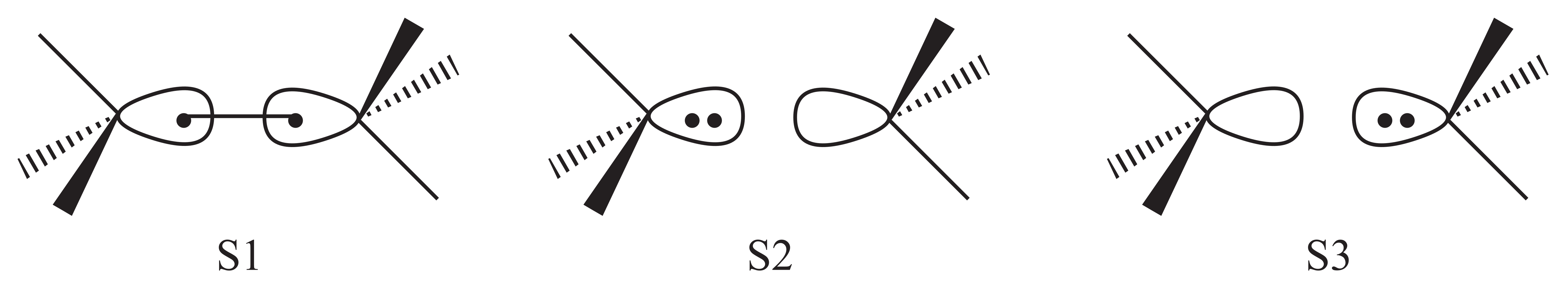
1.4.1. VB structures
3 VB structures are used in the computation for the active space including 2 orbitals and 2 electrons. The structures are shown in the following figure. S1 is the covalent structure in which electrons are shared in the two CH3 fragments, and S2 and S3 are two ionic structures in which eletrons belong to a certain fragment. Since the two CH3 fragments are qeuivalent, we expect that their weights should be the same.
1.4.2. Input file
The input file is shown below. The initial guess used in this computation can be obtained here.
Tip
The initial guess is provided as a section in XMVB input file. To provide initial guess for this computation, download the file including initial guess, copy the content and append it to the input file.
For cloud computation, this should be done after the input file is uploaded or the content is pasted to the input area.
C2H6 L-VBSCF
$ctrl
str=full nao=2 nae=2 iscf=5 iprint=3
orbtyp=hao frgtyp=atom
int=libcint basis=cc-pvdz
guess=read
$end
$orb
4*10
1-4
1-4
1-4
1-4
5-8
5-8
5-8
5-8
1-4
5-8
$end
$geo
C             0.0000000000000           0.0000000100000           0.7620840000000
H             0.0000000000000           1.0168937800000           1.1584307200000
H             0.8806558500000          -0.5084468900000           1.1584307200000
H            -0.8806558500000          -0.5084468900000           1.1584307200000
C            -0.0000000000000          -0.0000000100000          -0.7620840000000
H            -0.8806558500000           0.5084468900000          -1.1584307200000
H             0.8806558500000           0.5084468900000          -1.1584307200000
H             0.0000000000000          -1.0168937800000          -1.1584307200000
$end
In this case, the geometry is obtained from the output of MLatom. Each orbital is localized on the corresponding CH3 fragment. To make the computation simpler, the fragments are built with atoms by specifying FRGTYP=ATOM. The $FRAG section is missing so the numbers in $ORB correspond exactly to the ordering in $GEO.
1.4.3. Computational result
After the job is submitted and done, one can find information such as the overlap and Hamiltonian matrices in VB structure basis, weights of VB structures, the optimized VB orbitals and population analysis in the XMO output file. The weights of VB structures are shown below:
       **  WEIGHTS OF STRUCTURES **

1     0.69380  **  1:8    9  10
2     0.15310  **  1:8    9   9
3     0.15310  **  1:8   10  10
The first structure, which corresponds to a covalent structure, is the dominant structure with a weight of about 0.69 while the summation of weights of the two ionic structures is around 0.31. Therefore, the VB calculation gives consistent conclusion that the C-C \(\sigma\) bond is a covalent bond as common sense.
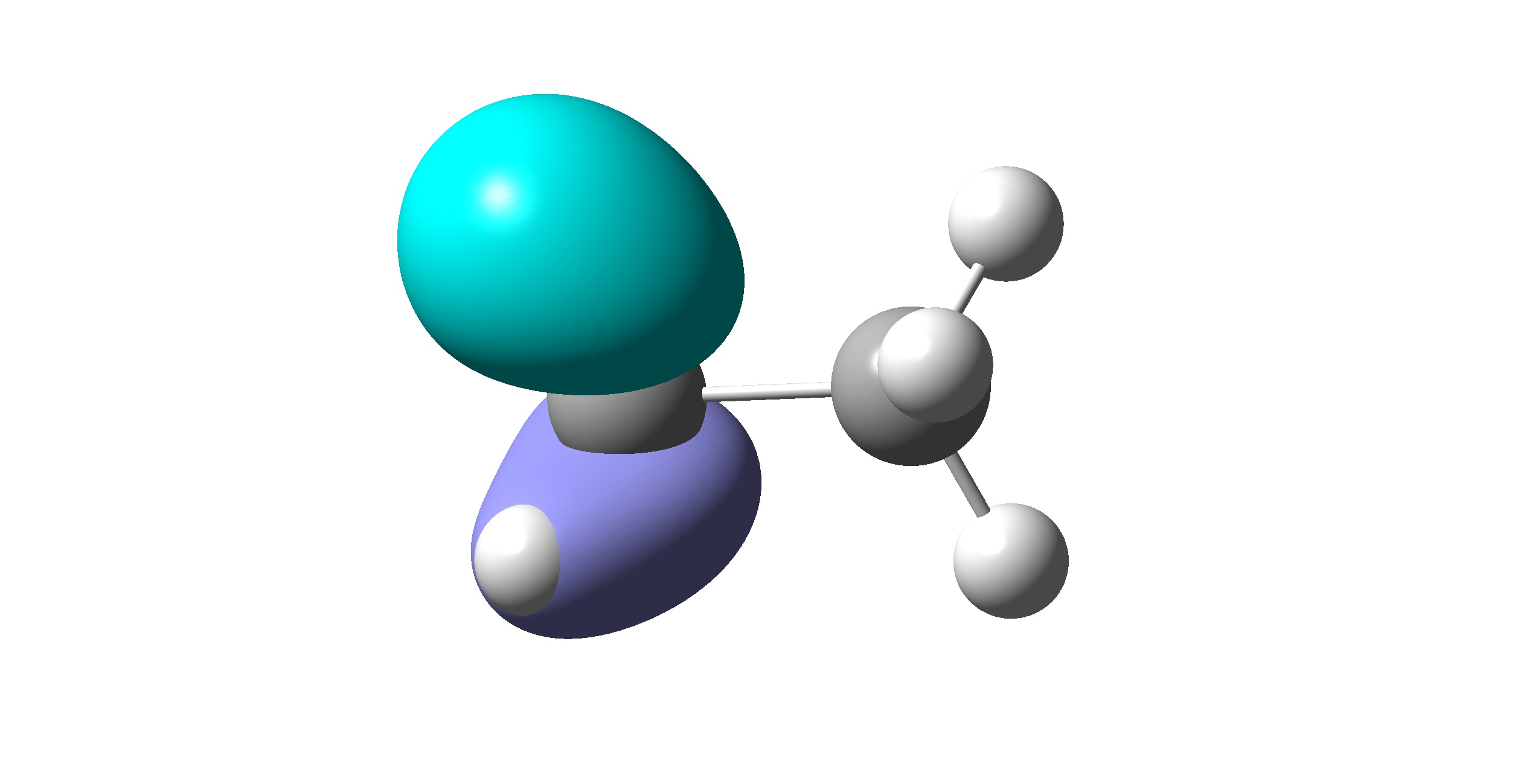
To confirm that the VB orbitals are correct, users may use the utility vbcubegen.exe to generate the cub file and visualize VB orbitals with programs such as MultiWfn, GaussView, etc. The visualized valence VB orbitals are shown in the following. Since the two CH3 fragments are equivalent, only orbitals on one fragment are shown. It is clear that all orbitals are correct and localized on the fragment.

VB orbital for 2\(s\)
VB orbital for 2\(p_y\)
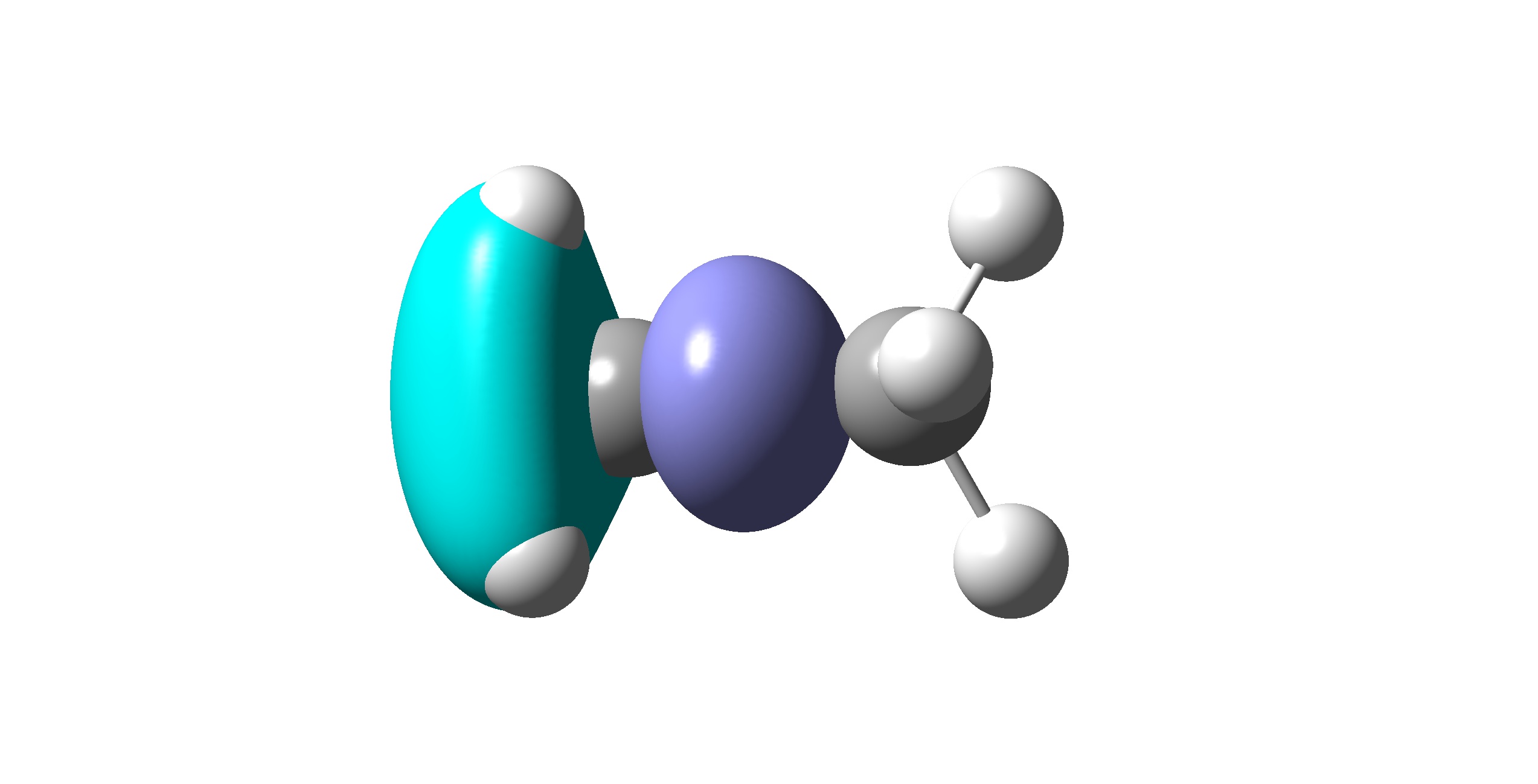
VB orbital for 2\(p_z\) constructing \(\sigma\) bond
1.4.4. Question
One may wonder if the C-C bond in ethane could be a charge-shift bond other than a conventional covalent bond. To rigorously figure out the type of the C-C bond, we then calculate the resonance energy (RE) of the C-C bond, and compare the resonance energy with corresponding bond dissociation energy (BDE=72.5 kcal/mol). What can we get from the ratio of RE and BDE? Is C-C bond in ethane a CSB?