4. Practice in machine learning with MLatom

This tutorial will use MLatom@XACS program. See its manual and tutorials for more details.

4.1. Machine learning model for H₂ potential energy curve

In this example, we will use a data set with full CI (FCI)/aug-cc-pV6Z energies along the potential energy curve of H₂ to train and use a kernel ridge regression (KRR) model.

4.1.1. Creating a kernel ridge regression model

Machine learning models can be created with MLatom by providing input and data files. In our example, we create a KRR model with Gaussian kernel (default) by providing the following input for MLatom:

createMLmodel                # Specify the task for MLatom
MLmodelOut=H2.unf            # Save model in H2.unf
XfileIn=R_451.dat            # File with R distances
Yfile=E_FCI_451.dat          # The file with FCI energies
sigma=opt                    # Optimize hyperparameter sigma
lambda=opt                   # Optimize hyperparameter lambda

This input requires two data files, one (R_451.dat) with input vector for KRR (here we just use internuclear distances in Å) and another (E_FCI_451.dat) with labels (reference FCI/aug-cc-pV6Z energies in Hartree). These files should be uploaded as auxiliary files to the XACS cloud computing platform.

After calculations finish, in your output file with .log extension, you should see lines similar to (numerical result can be slightly different):

CREATE AND SAVE FINAL ML MODEL

Analysis for values
Statistical analysis for 451 entries in the training set
MAE =           0.0000065324984
MSE =           0.0000002715356
RMSE =           0.0000111060390
mean(Y) =          -1.0360545152568
mean(Yest) =          -1.0360542437212
correlation coefficient =           0.9999999801933
linear regression of {y, y_est} by f(a,b) = a + b * y
    R^2 =           0.9999999603867
    a =          -0.0000018248557
    b =           0.9999979765628
    SE_a =           0.0000097455789
    SE_b =           0.0000093928306
largest positive outlier
    error =           0.0000546175797
    index = 5
    estimated value =          -1.1306260824203
    reference value =          -1.1306807000000
largest negative outlier
    error =          -0.0001005967022
    index = 1
    estimated value =          -1.1042329967022
    reference value =          -1.1041324000000

FINAL ML MODEL CREATED AND SAVED

4.1.2. Using the model

You can use the model created in the previous step for making predictions, in our case for new internuclear distances. Here, try to find bond length in H₂ through a simple 1D grid search. For this, you may use this input:

useMLmodel                   # Specify the task for MLatom
MLmodelIn=H2.unf             # Read in model from H2.unf
XfileIn=R_pred.dat           # File with R distances
YestFile=E_est.dat           # The file with ML-estimated energies

4.1.3. Questions

What is the bond length in H₂?
How much time did it take to finish calculations?

Note

Compare your result to experimentally known bond length of 0.7414 Å. Also, to the optimized geometry with the bond length of 0.7415 Å at the reference FCI/aug-cc-pV6Z level which took 5 CPU-days.

4.2. Choosing the right machine learning potential

MLatom provides a host of powerful machine learning potentials via native implementations and interfaces to third-party programs:

kernel methods for single-molecular PES:
- KREG (native). See tutorial. Can only be used for single-molecule PES.
- KRR-CM (KRR with Coulomb matrix, native).
- sGDML (through sGDML). Can only be used for single-molecule PES
neural network methods applicable to creating PES for different molecules:
- ANI (through TorchANI)
- DeepPot-SE and DPMD (through DeePMD-kit)
- GAP–SOAP (through GAP suite and QUIP)
- PhysNet (through PhysNet)

The choice of a suitable potential is not trivial. MLatom can help along by providing different ways of judging its accuracy. To evaluate an ML model’s performance, we need to test it with unseen data. MLatom provides estAccMLmodel task to do so for you by splitting the data set into the training and test sets.

Here we demonstrate how to evaluate the generalization error for building the machine learning potential of ethanol by training only on energies. We use a very small data set with 100 points for fast demonstration. You may need thousands of points for a real application.

We will test two machine learning potential models (see this paper for details):

KREG (based on kernel ridge regression and global descriptor),
ANI (based on neural network and local descriptor).

4.2.1. Testing a KREG model

Here is a sample input for it:

estAccMLmodel                            # Specify the task for MLatom
MLmodelType=KREG                         # Specify the model type (here - KREG)
XYZfile=ethanol_geometries.xyz           # File with XYZ geometries
Yfile=ethanol_energies.txt               # File with reference energies
sigma=opt                                # Optimize hyperparameter sigma
lambda=opt                               # Optimize hyperparameter lambda

Necessary data files with XYZ geometries ethanol_geometries.xyz and energies ethanol_energies.txt (reduced MD17 data set).

4.2.2. Questions

What are the errors in the training and test sets.
Is it enough to use training errors for evaluating the accuracy of the ML model?

4.2.3. Testing ANI-type model

In MLatom, except for the KREG model, we can also use other MLP models, e.g., ANI model (you can also try PhysNet or DPMD):

estAccMLmodel                            # Specify the task for MLatom
MLmodelType=ANI                          # Specify the model type
XYZfile=ethanol_geometries.xyz           # File with XYZ geometries
Yfile=ethanol_energies.txt               # File with reference energies

4.2.4. Question

Can you draw a conclusion whether the KREG or ANI model is more accurate?

4.2.5. Learning curves

Comparing models just based on their performance for a test set after being trained on the same data set is not enough to claim that one model is better than another. Performance of models can change when you change the size of the data set. Thus, ML models’ performances should be compared by evaluating their generalization error over different training set sizes and MLatom provides learningCurve task to automatically perform such calculations and summarize the results.

You can use the following input:

learningCurve                            # Specify the task for MLatom
MLmodelType=KREG                         # Specify the model type
XYZfile=ethanol_geometries.xyz           # File with XYZ geometries
Yfile=ethanol_energies.txt               # The file with reference energies
sigma=opt                                # Optimize hyperparameter sigma
lambda=opt                               # Optimize hyperparameter lambda
lcNtrains=10,25,50,75                    # Specify the number of training point to be examined
lcNrepeats=10,8,5,3                      # Specify the number of repeats for each Ntrain

MLatom prepares for you several csv files of the learning curve results in the folder named by your modeltype in the learningCurve directory.

E.g. this is a lcy.csv that recodes the learning curve of RMSE on energies, which can be visualized by suitable programs such as Excel:

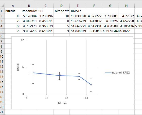
_images/lcy.png — Learning curve for the KREG model tested on the ethanol molecule

4.2.6. Questions

Why do you need repeating calculations (see Nrepeats for the number of repeating calculations) for each number of training points (Ntrain)?
Do you expect that errors drops stronger when you increase training set a) from 100 to 1000 or b) from 1000 to 2000 training points?