1. Manual
1.1. Overview
1.1.1. Methods
XMVB provides an ab initio computing platform for various VB approaches, including classical VB methods, such as VBSCF, BOVB, VBCI, VBPT2, modern VB methods, such as SCVB and GVB, and molecular orbitals based VB method, BLW. Combined with solvation models, it can perform VBPCM, VBEFP, and VBSMD to account for solvent effects. Incorporating XMVB with KS-DFT code, it can be applied to hybrid DFVB calculation. In this manual, only a brief introduction to classical VB methods is provided. Please read the following references for details:
Articles:
Book Chapters:
1.1.1.1. The VBSCF method
The wave function of Valence Bond Self Consistent Field (VBSCF) method is the linear combination of VB structures, as shown below.
In VBSCF method, All VB structures share the same set of VB orbitals, and both sets of the structure coefficients and VB orbitals are optimized simultaneously to minimize the total energy. This is comparable to the MCSCF method in the MO theory. VBSCF method takes care of the static electron correlation and gives equivalent results to the MO-based CASSCF calculations. It should be noted that the dynamic electron correlation is not accounted for in the VBSCF method. In XMVB, VBSCF method is the default method, thus this keyword can be ignored.
1.1.1.2. VB Methods including Dynamic Correlation
The VBSCF result includes only static correlation energy, which makes VBSCF results not accurate enough for quantitative researches. The purpose of post-VBSCF methods is to take dynamic correlation into account as much as possible to get accurate enough results. There are several post-VBSCF methods developed so far and will be introduced in this section. It is strongly recommended to perform post-VBSCF calculations with initial guesses from a pre-proceeded VBSCF calculation. As to VBCI and VBPT2, this is enforced.
1.1.1.2.1. The BOVB method
The orbitals of Breathing Orbital Valence Bond (BOVB) method are also optimized by SCF procedure, as VBSCF does. The difference between VBSCF and BOVB methods is that BOVB provides an extra degree of freedom during orbital optimization. In BOVB method, each VB structure has its own set of orbitals and are optimized independently
Thus, the orbitals adopt themselves to the instantaneous field of the VB structures, rather than to the mean field of all the structures in VBSCF. This degree of freedom makes the orbitals in BOVB “breathing” in different structures, introduces dynamic correlation, and thereby improves considerably the accuracy of VB computations.
1.1.1.2.2. The VBCI method
The VBCI method is based on localized VB orbitals. In this method VB orbitals are divided to several blocks (occupied and virtual orbitals). Excited VB structures are generated by replacing occupied VB orbitals with virtual orbitals that are localized on the same block. The wave function of VBCI is the linear combination of all reference and excited VB structures
where \(\Phi^i_K\)is CI structure coming from VBSCF structure K, including reference and excited structures, and the coefficients \({C_{Ki}}\) are obtained by solving the secular equation. The VBCI weight can be given either with equation
which gives weights of all CI structures, or in a more compact way as
where \(W_K\) is the contracted weights of reference structure K, including weights of all CI structures coming from structure K.
Allowing for different excitations for different electronic shells, currently the VBCI method consists of the following calculation levels:
VBCI(S,S): only single excitations are involved in either active electron or inactive electron. In brief, this is a VBCIS procedure.
VBCI(D,S): the active shell is treated by single and double excitations, whereas the inactive shell by single excitations only. Also included in this level are double excitations which consist of a single excitation from each shell.
VBCI(D,D): single and double excitations are involved for both active and inactive electrons, in short, VBCISD.
1.1.1.2.3. The VBPT2 Method
Another post-VBSCF method is Valence Bond second-order Perturbation Theory (VBPT2) method. The wave function of VBPT2 can be separated into 2 parts as
where VBSCF wave function is taken as the zeroth-order wave function \(\Psi^0\), and the first-order part is the combination of singly and doubly excited wave functions
To enhance the efficiency of VBPT2, the virtual orbitals are delocalized and orthogonal to the occupied space, and the excitations include all virtual orbitals. In this manner, the excited structures in VBPT2 don’t belong to any fundamental structure, and the matrix elements can be calculated easily with Coulson-Slater rules.
1.1.2. Installation
Both distributions of XMVB are currently available for LINUX platform. 1.5GB RAM is required. Followings are the instructions for installation. Note that the source code will NEVER be released to the users. Only compiled object file or executable files are available for users.
XMVB 4.0 is released as a package of compiled executable files. To install the stand-alone distribution, the users should unpack the compressed tar file by using the following command,
tar xvfz xmvb.tar.gzOnce the file is unpacked successfully, a new directory xmvb/ will be created.
1.1.3. Running a job
The user may run XMVB job with simple command
xmvb.exe file.xmi
The output will be printed to the screen. To redirect the output to an output file, the user may use pipeline like:
xmvb.exe file.xmi > file.xmo
or
xmvb.exe file.xmi | tee file.xmo
For the parallelization in XMVB, see below.
1.1.3.1. Parallelization in XMVB
The OpenMP parallelization is supported by XMVB. It provides efficient parallelization in the node. By default, XMVB runs jobs in serial. To run XMVB with multiple cores, the user may run the job with command
xmvb.exe -n NP file.xmi
where NP is the number of processors / cores for parallelization.
For large systems, OpenMP parallelzation may proceed a strange “segmentation fault”. This is because the stack size of threads is not large enough. This can be avoided by setting the stack size to a certain number to avoid this error. In OpenMP parallelization, the stack size of master and slave threads are set in different ways. The stack size of master thread is set by command ulimit as shown
ulimit -s stack_size
The default stack size is 8192. Setting a larger value or simply
ulimit -s unlimited
The stack size of slave threads are controlled by environment variable $OMP_STACKSIZE. Following command will set the stack size of each slave threads to 1GB
export OMP_STACKSIZE=1G
1.1.3.2. Basis sets in XMVB
Currently user-defined basis sets and pseudopotential are not supported by XMVB yet. Users can only define one basis set in the computation. Following basis sets are supported by XMVB so far:
Pople basis sets, such as STO-6G, 6-31G, 6-311+G**, etc.
Dunning’s basis sets, including cc-pVXZ and aug-cc-pVXZ (X=D,T,Q,5,6).
Ahlrich’s basis sets, including def2-SVP, def2-SVPD, def2-TZVP, def2-TZVPD, def2-TZVPP, def2-TZVPPD, def2-QZVP, def2-QZVPD, def2-QZVPP, def2-QZVPPD.
1.1.4. Utilities
Tip
This utilities in this section is not provided on the XACS cloud computing platform.
1.1.4.1. Viewing VB orbitals: Moldendat
Viewing VB orbitals is available. To do that, you need to run a utility, called “moldendat”:
moldendat.exe MOfile vbdat [denfile] >&vbfile
where MOfile is an output file of Gaussian or GAMESS-US, or formatted Gaussian checkpoint file (.fchk); vbdat is a XMVB xdat file; if .fchk file is inputted, an optional XMVB density file with extension “.den” is also supported. The program will produce an NEW output file (vbfile) with the same format as input MO files, with which you can view VB orbitals with MOLDEN or MacMolPlt (for GAMESS-US only) packages.
1.1.4.2. Cartesian to spheric integral transformation: 6D25D
This utility transforms integrals from cartesian type to spheric (harmonic) type. Currently the utility supports D and F transformation only and not available for higher basis functions.
To run the utility, typing the command as following:
6d25d.exe [-if gau/gms/lib] [-of gau/std]
where option -if defines the sequential of cartesian F functions. Argument gau means the sequential in Gaussian, gms means the sequential in GAMESS-US. Option and “lib” means the sequential by LIBCINT; -of defines the output format of spheric F basis functions. Argument gau means the spheric F functions used in Gaussian package and std means standard spheric F function, which is different from the definition in Gaussian. By default, 6d25d will use Gaussian type for both input and output format.
After running 6d25d, the original cartesian integral files x1e.int, x2e.int and INFO will be overwritten by the spheric integrals. Make a backup of your cartesian integral files if you need them later.
1.1.4.3. Use NBOs as XMVB initial guess: NBOPREP
This utility read the NBOs obtianed from a previous GAMESS/Gaussian calculation, and transfer them to the XMVB readable formats so that user may use them as initial guess in later XMVB calculations with keyword GUESS=NBO.
The user need to run a GAMESS/Gaussian calculations with keyword
$NBO PLOT $END
to get files with name FILE.36 and FILE.37 which stores NBOs and PNBOs. Then run NBOPREP as following:
nboprep.exe outfile [NBO/PNBO]
where “outfile” refers to the output file of GAMESS/Gaussian program, and “NBO/PNBO” tells the program which kind of NBOs should be prepared for later XMVB calculation. The user may be able to use keyword GUESS=NBO by copying file “orb.nbo” generated by NBOPREP to the directory where the XMVB job will be proceeded.
1.1.4.4. Generate cube file for XMVB computation: vbcubegen
This utility generates cube grid file to visualize VB orbitals with other programs. It supports module distribution or stand-alone XMVB with keyword INT=CALC or INT=LIBCINT since basis function information is essential for generating grids. The syntax of this utility is
vbcubegen.exe xmofile
where xmofile refers to the XMO output file of the XMVB computation. After that, a cube grid file with the same file name as the xmo file will be generated, with which the user may visualize VB orbitals with programs such as GaussView, Multiwfn etc.
1.2. Input
The extension name of XMVB input file is “xmi”. All the contents is organized in sections and case insensitive. The input file is structured in sections with following rules:
The first line of an xmi file is the job title or description of the job and should not be replaced or omitted.
A section start with a line includnig only the section name and ends with a line with only “$END”.
All contents after “#” is recognized as a comment and will not be parsed.
Commonly used sections are:
A typical example of XMVB input file is shown below. The user may download the input file with detailed explaination here.
H2 L-VBSCF
$CTRL
VBSCF
NSTR=3
NAO=2 NAE=2
ORBTYP=HAO FRGTYP=SAO
INT=LIBCINT
BASIS=CC-PVTZ
$END
$STR
1 2
1 1
2 2
$END
$FRAG
1 1
SPZDXXDYYDZZ 1
SPZDXXDYYDZZ 2
$END
$ORB
1 1
1
2
$END
$GEO
H 0.0 0.0 0.0
H 0.0 0.0 0.74
$END
$GUS
15 15
# ORBITAL 1 NAO = 15
-0.3532245024 1 -0.5363311264 2 -0.2343104477 3 -0.0000000000 4
 0.0000000000 5 -0.0199961314 6 -0.0000000000 7  0.0000000000 8
-0.0192894825 9 -0.0003896018 10 0.0000000000 11 -0.0000000000 12
-0.0003896018 13 0.0000000000 14 -0.0020820012 15
# ORBITAL 2 NAO = 15
 0.3532245024 16 0.5363311264 17 0.2343104477 18 0.0000000000 19
-0.0000000000 20 -0.0199961314 21 0.0000000000 22 -0.0000000000 23
-0.0192894825 24 0.0003896018 25 -0.0000000000 26 -0.0000000000 27
0.0003896018 28 0.0000000000 29 0.0020820013 30
$END
1.2.1. Global control ($CTRL)
The $CTRL section contains the information of how a job is performed. The input format is name=value or name=option, except for the keywords which need no values or options. <enter> and <space> are used to separate keywords. If a keyword accepts several options in a time, the options are separated with “,”.
1.2.1.1. Keywords for Global Control
1.2.1.1.1. UNIT=option
The unit for geometry in $GEO. Available options are:
* ANGS: Geometry is given in Angstroms. This is the default option.
* BOHR: Geometry is given in Bohr.
1.2.1.1.2. ITMAX=n
n is the maximum number of iterations. Default value is 200.
1.2.1.1.3. NMUL=n
n is the spin multiplicity (2S + 1) of system. Default value is 1, which means singlet state.
1.2.1.1.4. NAO=m
m is the number of active VB orbitals whose occupation number varies in the structures. NAO is required if keywords STR or ISCF=5 (see below) is specified.
1.2.1.1.5. NAE=n
n is the number of active VB electrons which occupy the active orbitals. NAE is required if keywords STR or ISCF=5 (see below) is specified.
1.2.1.1.6. NSTR=n
n is the number of VB structures (or determinants). This keyword can be omitted if STR (see below) is assigned.
1.2.1.1.7. STR=options
This keyword generates VB structures automatically and hence NSTR and the $STR section are not needed. This keyword requires NAO and NAE to declare the active space. Users may use one or several of the following options:
COV: Covalent structures will be generated.
ION[(n-m)]: Ionic structures will be generated. A simple ION will generate all ionic structures; ION(n,m) will generate only the \(n^\textrm{th}\) and \(m^\textrm{th}\) order ionic structures and ION(n-m) will generate ionic structures from the \(n^\textrm{th}\) to the \(m^\textrm{th}\) order.
FULL: All VB structures will be generated.
1.2.1.1.8. FIXC
Request to fix structure coefficients for VB structures. In VB theory, the coefficients are obtained by solving the secular equation
For some special purposes, one may want to fix the coefficients. In such situation, the coefficients are inputted following the corresponding VB structures and the energy will be obtained directly by
For example, the following input will constrain the coefficients of the three VB structures to be 1.0:0.5:0.5
$STR
1 2 1.0
1 1 0.5
2 2 0.5
$END
The corresponding wave function will in the expression
where N is the normalization coefficient.
1.2.1.1.9. GROUP=EXP
Divide VB structures into groups according to the expression EXP. An expression with n structures divided into m groups can be expressed as:
Here \(S_{i1} \ldots S_{nm}\) are the structure numbers, a comma “,” is used to separate the structures numbers in the same group, and two commas “,,” is used to separate different groups. Coefficients of structures should be given in Global control ($CTRL), similar to FIXC. The ratio of VB structures within the same group will be fixed, as introduced in FIXC. The coefficients of VB structures in different groups will not be fixed and shall be optimized by solving secular equation. Following is an example:
$CTRL
NSTR=3
GROUP=1„2,3
$END
$STR
1 2 1.0 # S1
1 1 0.5 # S2
2 2 0.5 # S3
$END
The above example devide 3 VB structures into 2 groups:
Group 1. \(G_1 = S_1\)
Group 2. \(G_2 = 0.5(S_2 + S_3)\)
Hence a 3 structure problem becomes a 2 “structure” problem:
where \(C_1\) and \(C_2\) are coefficients of \(G_1\) and \(G_2\) obtained by solving secular equation. The finalwave function can be expressed as
1.2.1.1.10. NSTATE=n
Energy, coefficients and weights of structures for the \(n^\textrm{th}\) excited state, rather than for the ground state, will be calculated and printed out. The values of n can be:
0: The ground state.(Default)
n: The \(n^\textrm{th}\) excited state.
Note
VB orbitals are optimized by minimizing the energy of required state. When the \(n^\textrm{th}\) excited state is requested, the \((n+1)^\textrm{th}\) root will be chosen as the \(n^\textrm{th}\) excited state when solving the secular equation. Thus, n must be smaller than the number of structures.
For VBCI calculaitons, NSTATE can be only 0 or 1.
1.2.1.1.11. SORT
Sort the VB structures in descending order according to coefficients.
1.2.1.1.12. CTOL=tol
Set the Coefficient TOLerance when printing coefficients and weights of VB structures.
Only the coefficients and weights of VB structures whose absolute values of coefficients are not smaller than tolerance tol will be printed. The default tolerance is 0, which means all structures will be printed.
Note
The tolerance tol is a real parameter. For instance,
CTOL=0.01
means that only structures whose absolute values of coefficients larger than or equal to 0.01 will be printed. For VBCI this keyword is not functioning
1.2.1.1.13. CICUT=n
Set cut threshold to \(10^{-n}\) for CI configurations. The contribution of a CI configuration is estimated by perturbation theory. If the contribution is less than the threshold, the configuration will be discarded. This will reduce the computational effort for CI calculations. Recommended values are 5 or 6. Default value is 0 (no cut).
1.2.1.1.14. NCOR=m
In VBCI or VBPT2 calculations, the first m orbitals (2m electrons) will be frozen in the VBCI or VBPT2 calculation. In BOVB caluclations, the first m orbitals will be kept as VBSCF orbitals. The default value is 0, which means all orbitals will be counted in VBCI, VBPT2 or BOVB.
1.2.1.1.15. GUESS=option
This keyword describes the way to generate or read the initial guess for a VB computation.
Valid options can be:
AUTO: The program automatically provides guess orbitals by diagonalizing a fragmant-localized Fock matrix. This is the default option.
UNIT: The first basis function of an orbital in $ORB is set to be the guess for the orbital.
MO: Initial guess will be obtained from MOs.
READ: Guess orbitals are read from external file, which should be provided by user.
Note
The Initial guess description ($GUS) section is required when
GUESS=MOorGUESS=READis specified. Note that the format of the Initial guess description ($GUS) section differs depending on whetherGUESS=READorGUESS=MOis used. Detailed explanations for both formats are provided in the Initial guess description ($GUS) section documentation.To enhance user convenience and ensure reliable calculations, the software automatically detects whether the format in the Initial guess description ($GUS) section corresponds to
GUESS=READorGUESS=MO. Therefore, if the Initial guess description ($GUS) section is included, theGUESSkeyword can be omitted when using either of these two options.
1.2.1.1.16. WFNTYP=option
Options for the way to expand the many-electron wave functions of system.
STR: VB structures are used. (Default)
DET: VB determinants are used for state functions, instead of VB structures.
1.2.1.1.17. ORBTYP=option
Specify the type of VB orbitals. Valid options are:
HAO: Hybrid Atomic Orbitals are used.
OEO: Overlap Enhanced Orbitals are used.
GEN: VB orbitals are defined by users. The orbitals will be described in terms of basis functions explicitly in Orbital description ($ORB) section. (Default)
Note
Fragments definition ($FRAG) is needed if
ORBTYP=HAOis specified. The Fragments definition ($FRAG) section will specify the fragments based on atoms or basis functions and orbitals will be assigned in Orbital description ($ORB) section based on the fragment definitions in Fragments definition ($FRAG).ORBTYP=OEOdoes not need Fragments definition ($FRAG) and Orbital description ($ORB) sections since the OEOs are delocalized in the whole system.ORBTYP=GENdoes not need Fragments definition ($FRAG) section.
1.2.1.1.18. FRGTYP=option
Specify the type of fragments when ORBTYP=HAO.
ATOM: The fragments of system will be defined with atoms. This is the default.
SAO: The fragments of system will be defined with symmetrized atomic orbitals.
Note
Fragments definition ($FRAG) is required for FRGTYP=SAO. For FRGTYP=ATOM, each atom is considered as a fragment if no FRAG section appears in the input file.
Tip
In addition to assigning all orbitals in the Orbital description ($ORB) section, the software supports a simplified input format that requires only the active orbitals to be assigned while using the default options for ORBTYP and FRGTYP. For more details, refer to the Active orbital description ($ACTORB) section.
1.2.1.1.19. FRZORB=EXP
Specify the indices of orbitals to be frozen. Frozen orbitals will not be optimized in the calculation. Following is an example for frozing orbital 1, 3, 5, 6 and 7
$CTRL
FRZORB=1,3,5-7
$END
Note
This keyword is only available for VBSCF calculation currently.
1.2.1.2. Keywords for Computational Methods and Algorithms
1.2.1.2.1. HF/RHF/UHF/ROHF
A Hartree-Fock calculation will be proceeded. RHF/UHF/ROHF represent the restricted, unrestricted and restricted open-shell Hartree-Fock calculations respectively. When only “HF” is assigned, RHF will be proceeded when system is singlet and UHF for other cases.
1.2.1.2.2. Density Functional Theory
A DFT calculation will be proceeded. Currently supported keywords and corresponding functionals are listed below:
- GGA Functionals
BLYP Becke88 + Lee-Yang-Parr XC functional
PBE Perdew-Burke-Ernzerhof XC functional
PW91 Perdew-Wang 1991 XC functional
- Hybrid Functionals
BHHLYP 0.5 B88 + 0.5 HFX + LYP hybrid functional
B3LYP Becke’s 3 parameter hybrid functional
B3LYP-D3 B3LYP with D3 dispersion correction
B3LYP-D3BJ B3LYP-D3 with damping
PBE0 A hybrid with 25% exact exchange and 75% DFT exchange made from PBE
The users may use “R”, “U”, and “RO” ahead of the name of functional to specify restricted, unrestricted or restricted open-shell calculations, the same as HF method. For example, “RB3LYP” will run the restricted B3LYP calculation. If only the name of functional is specified, restricted calculation will be run for singlet and unrestricted for others.
1.2.1.2.3. VBSCF
A VB Self-Consistent Field computation is requested. This is the default method for the XMVB program.
1.2.1.2.4. BOVB
Ask for a Breathing Orbital VB (BOVB) calculation.
Note
BOVB method cannot be used with VBCI.
BOVB method is usually more difficult to converge than VBSCF. Thus, it is recommended to run a BOVB job with a good initial guess. It is recommended to run a VBSCF calculation first, followed by the BOVB calculation with optimized VBSCF orbitals as the initial guess.
1.2.1.2.5. VBCIS:
Ask for a VBCIS calculation.
1.2.1.2.6. VBCISD
Ask for a VBCISD calculation.
1.2.1.2.7. VBPT2
A VBPT2 computation will be performed.
1.2.1.2.8. HC-DFVB=func
Ask for an HC-DFVB calculation. func is the DFT functional used for DFVB computation. Currently BLYP, B3LYP, B3LYP5, BHHLYP, PW91, PBE, and PBE0 functionals are available.
1.2.1.2.9. LAM-DFVB=func
Ask for an λ-DFVB(U) calculation. func is the DFT functional used for DFVB computation. Currently only BLYP functional is available.
1.2.1.2.10. MS-DFVB=func
Ask for an λ-DFVB(MS) calculation. func is the DFT functional used for DFVB computation. Currently only BLYP functional is available. Additionally, MS-DFVB has to be used with keyword WSTATE.
Note
The parameters used in the λ-DFVB(U) and λ-DFVB(MS) methods are specifically fitted for the VBSCF wave function of all structures with OEOs. Therefore, it is recommended to use STR=FULL and ORBTYP=OEO together with LAM-DFVB or MS-DFVB. While other combinations of STR and ORBTYP may also work with LAM-DFVB or MS-DFVB, these are not recommended, as no parameters are available for other wavefunction types.
1.2.1.2.11. TBVBSCF
Activate tensor-based VBSCF. Currently TBVBSCF is valid only when:
ISCF=5,NAO=mandNAE=nare selected.Structures are generated automatically with STR=options.
Number of active electrons should be at least 4, in which 2 for both \(\alpha\) and \(\beta\) parts.
1.2.1.2.12. ISCF=n
ISCF specifies orbital optimization algorithm. The value n currently can be:
2: Analytical gradients in terms of basis functions with the L-BFGS algorithm. This algorithm involves only the first-order density matrix and is the default for BOVB.
5: Analytical gradients in terms of VB orbitals with the L-BFGS algorithm. This is the most efficient algorithm so far. Keywords
NAOandNAEare needed. This is the default for VBSCF.6: VBSCF with full hessian matrix.
NAOandNAEare needed for this option. This algorithm is potentially faster and more robust than ISCF=5, but it is still under development and thus is not recommended in the current version of the program.
1.2.1.2.13. WSTATE=EXP
Activate the state-average VBSCF/BOVB calculation. WSTATE may provide an array containing non-zero weights of the specific states. Following is the example for
$CTRL
NSTR=10 WSTATE(3)=0.5,0.0,0.3,0.0,0.0,0.2
$END
Note
WSTATE currently cannot be used with TBVBSCF and ISCF=6.
1.2.1.3. Keywords for Integrals
1.2.1.3.1. INT=option
Read integrals from file or calculate them directly. The valid options can be:
LIBCINT: Integrals are calculated directly by an external library LIBCINT. Section Geometry description ($GEO) is essential. This is the default option.
RI: 2-e integrals are evaluated with resolution identity (RI).
COSX: 2-e integrals are evaluated with grid-based COSX.
READ: Read integrals from existing files “x1e.int”, “x2e.int” and “INFO”.
Note
Note that he absolute energies vary depending on the integral type used. Therefore, ensure that the relative energy is calculated using the same integral type for consistency.
1.2.1.3.2. BASIS=basis_set
Assigning the basis set when INT=CALC is requested. Basis sets are expressed the same way as Gaussian, i.e. 6-31G*, aug-cc-pVTZ etc. The supported basis sets can be found in Basis sets in XMVB.
1.2.1.3.3. NCHARGE=n
Charge of the system in current XMVB calculation. Default is 0, which means the neutural system. Positive numbers denote a cation system and negative numbers mean the system is anion. This keyword will also specify the number of electrons in current calculation, NEL is not needed anymore in such case.
1.2.1.4. Keywords for Wave Function Analysis
1.2.1.4.1. BOYS
Boys localization is requested for the final VB orbitals.
Note
It is strongly recommended to use this keyword for VBSCF. This makes VB orbitals easier to be interpreted and more physically meaningful.
Boys localization is available only for VBSCF method.
Boys localization can be only used in cases in which orbitals are separated into blocks, and there is no common basis function between blocks.
1.2.1.4.2. OUTPUT=AIM
WFN file for AIM2000 program will be printed. A $AIM with WFN filename is relevant for this keyword. This is not available if INT=READ is assigned.
1.2.1.4.3. MOLDEN
MOLDEN file will be punched with name input.molden in which input is the input file name. This file can be used to visualize the geometry and VB orbitals. Cannot be used with INT=READ.
1.2.1.4.4. VBCAD[=option]
Diabatization procedure VBCAD will be proceeded after VBSCF or BOVB computation. Currently only 2-state diabatization is supported. VBCAD separates two diabatic states by maximizing the weights different of VB structures.
Users may use one of the following options:
C2: The square of coefficients of VB structures will be used instead of weights of VB structures. This is the default option.
CC: The Coulson-Chirgwin weights will be used.
RE: The Renormalize weights will be used.
LOWDIN: The Löwdin weights will be used.
INV: The Inverse weights will be used.
n: Input number instead of name of weights.
1is a synonym ofC2,2is a synonym ofCC,3is a synonym ofRE,4is a synonym ofLOWDIN,5is a synonym ofINV.
1.2.1.4.5. CADGRID=n
The step size for searching the givens rotation angle that maximizing the weights different of VB structures in degree. The default is 0.5 degree.
Note
The keyword CADGRID needs to be used together with VBCAD. However, the default options has been extensively used and they all result in well-separated diabatic states. So it is recommended to simply use the VBCAD keyword alone.
The CADGRID keyword is intended to be used with VBCAD. However, due to the extensive use of default settings, which result in well-separated diabatic states, it is recommended to use the VBCAD keyword on its own.
1.2.1.5. Keywords for Geometry Optimization
Following are the keywords for geometry optimization. Keywords in this section is only available for VB computations with INT=LIBCINT. Currently only global minima optimization with no constraint is supported.
1.2.1.5.1. OPT
A geometry optimization will be performed in Cartesian coordinates. Currently geometry optimization is only available for the VBSCF method (ISCF=5 or ISCF=6).
1.2.1.5.2. HESS=option
Options for evaluating initial Hessian used in geometry optimization. Currently following options are available:
GUESS: Initial Hessian is evaluated by a “guess” procedure based on some empirical parameters. This is the default option.
SEMINU: A semi-numerical procedure is used to evaluate initial Hessian. In this procedure, the gradient is evaluated analytically and Hessian is numerical based on analytical gradients.
FULLNU: A fully numerical procedure is used to evaluate initial Hessian. Both Hessian and gradient will be evaluated in purely numerical way.
1.2.1.5.3. MAXCYCLES=n
The maximum cycles for geometry optimization. The default is the maximum between 20 and 6*N, where N is the number of atoms.
1.2.1.5.4. GRADIENT
Geometrical gradient will be evaluated for current geometry but not for optimization.
1.2.1.5.5. Geometry optimization using Gaussian’s optimizer
To enable geometry optimization using Gaussian’s optimizer, use the keyword OPT=GAUSSIAN(NOMICRO[, ...]). The option NOMICRO activates a faster optimization approach and is recommended. The options within the parentheses correspond to those of the Opt keyword in Gaussian. When using Gaussian’s optimizer for geometry optimization, the Geometry description ($GEO) section must be provided in Gaussian format. The format for specifying fixed atoms or variables is the same as in Gaussian. Below is an example for optimizing the HCN molecule using internal coordinates, where the bond length B2 and bond angle A1 are held fixed, while bond length B1 is optimized.
$CTRL
OPT=GAUSSIAN(nomicro,z-matrix)
$END

$GEO
H
C   1  B1
N   2  B2  1  A1

B1=1.07

B2=1.1466
A1=179.999
$END
Note
This keyword is available on the XACS cloud only.
1.2.2. VB Structure description ($STR)
The $STR section describes the information of VB structures or VB determinants if DET of $CTRL section is specified. For VB structures, paired electrons, which may be lone pairs or covalent bonds, should be written first followed by unpaired electrons. The number of unpaired electrons depends on the spin multiplicity. For example: For a structure with three lone pairs (orbitals 1, 2, and 3), one covalent bond (orbitals 4 and 5), and one unpaired electron (orbital 6), the structure is expressed as,
1 1 2 2 3 3 4 5 6
For determinants, all alpha orbitals are listed first, followed by beta orbitals. For example: A determinant of alpha orbtials 1, 2, 3, 4, and 6 and beta orbtials 1, 2, 3, and 5 is expressed as
1 2 3 4 6 1 2 3 5
Note that it is strongly recommended to write the most important structure as the first one.
This can avoid potential problems in VBCI.
If BOVB is specified in $CTRL section, the program will try to convert the VB orbitals into breathing orbitals. It uses automatically different orbitals for different structures. For example: If the initial VB structures are:
1 1 2 3
1 1 2 4
1 1 3 5
The program will convert them to:
1 1 2 3
6 6 7 4
8 8 9 5
Note that the VB structures should be independent. VB structures are recommended to be written in the following orders:
Inactive Active
where “Inactive” stands for the inactive orbitals which keep doubly occupied in all structures; “active” stands for the active orbitals whose occupation varies in the structures. The singly occupied orbitals in high-spin systems should always be put in the tail of the structures.
Following are the examples of typical bonding patterns and their corresponding VB Structure description ($STR) and Global control ($CTRL) sections, in which only active orbitals are labeled:
System of 2-electrons on 2-centers
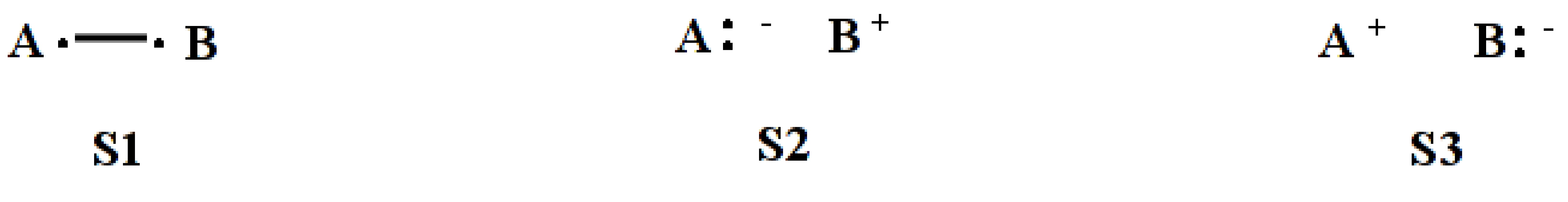
$CTRL
nstr=3 nmul=1
$END
$STR
1 2 ; S1
1 1 ; S2
2 2 ; S3
$END
System of 3-electrons on 2-centers
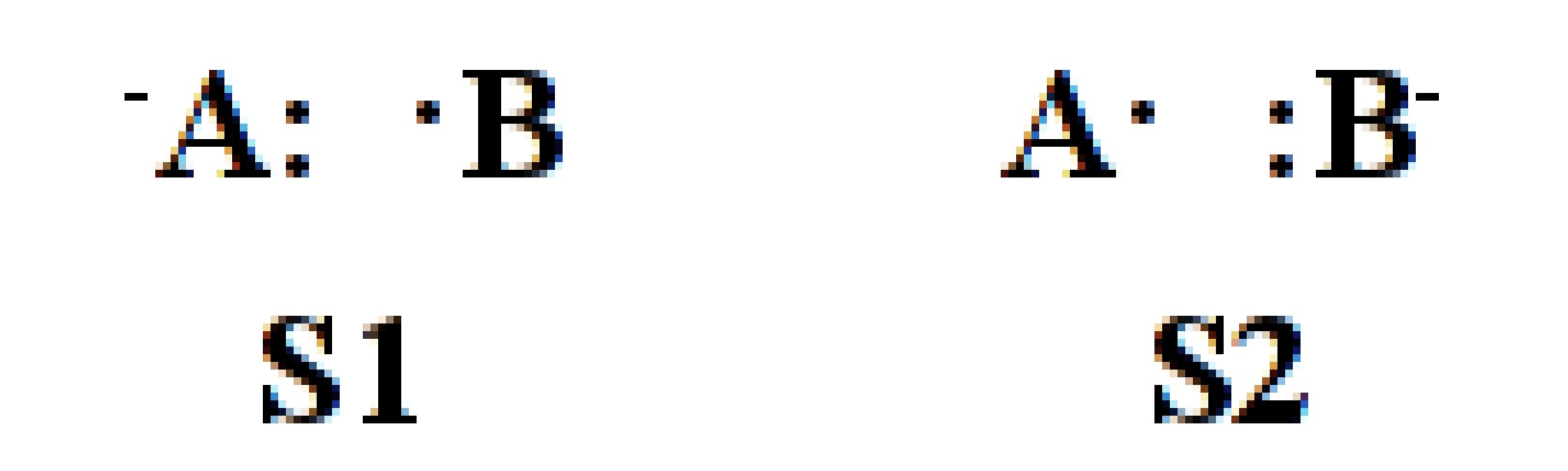
$CTRL
nstr=2 nmul=2
$END
$STR
1 1 2 ; S1
2 2 1 ; S2
$END
System of 3-electrons on 3-centers
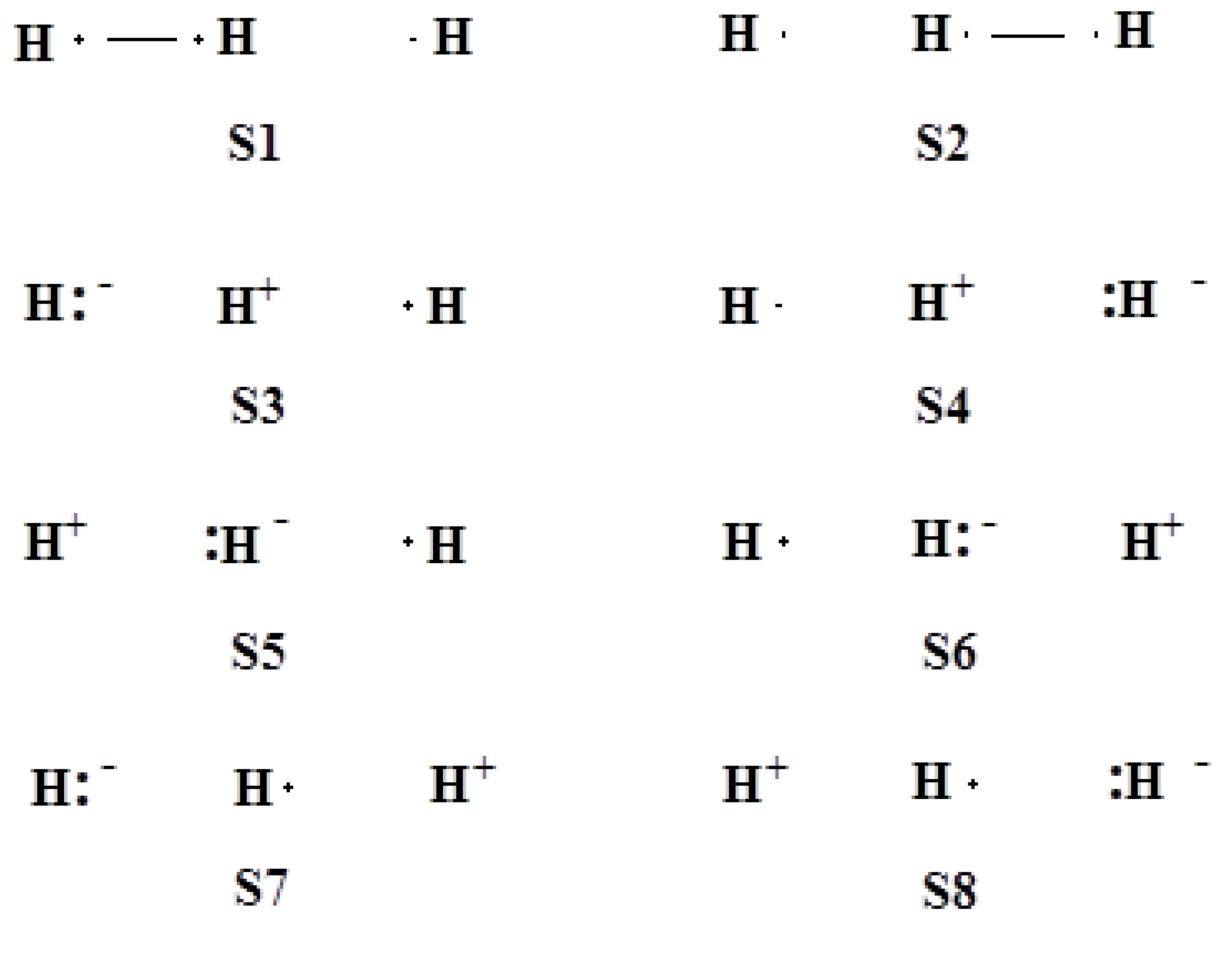
$CTRL
nstr=8 nmul=2
$END
$STR
1 2 3 ; S1
2 3 1 ; S2
1 1 3 ; S3
3 3 1 ; S4
2 2 3 ; S5
2 2 1 ; S6
1 1 2 ; S7
3 3 2 ; S8
$END
System of 4-electrons and 3-centers
6 VB structures (3 VB orbitals with 4 electrons, singlet)
$CTRL
nstr=6 nmul=1
$END
$STR
1 1 2 3 ; S1
1 1 2 2 ; S2
1 1 3 3 ; S3
1 2 3 3 ; S4
2 2 3 3 ; S5
2 2 1 3 ; S6
$END
Note
- In XMVB 4.0, VB structures are represented in a new style in the output file for better readability. For VB structures, the inactive part is shown in the format of “1:X”, where “X” is the number of inactive orbitals. In the active part, ionic pairs are shown in the format “X X” where “X” is the doubly occupied orbital, and a covalent bond is shown as “X-Y”, where “X” and “Y” are orbitals between which covalent bonding is made. High spin electrons (if there are) are always shown at last.
For example, the covalent structure “2 2 1 3” will be shown as 2 2 1-3 in the output file.
1.2.3. Fragments definition ($FRAG)
Generally, the $FRAG section is required if ORBTYP=HAO. In this section, fragments in which VB orbitals are localized will be defined and the orbitals will be generated with the basis functions specified in the fragments.
The syntax of $FRAG is:
$FRAG
nf(1), nf(2), . . . nf(N)
[basis function description(1)] lf(1,1), lf(2,1), . . . lf(nf(1),1)
[basis function description(2)] lf(1,2), lf(2,2), . . . lf(nf(2),2)
. . .
[basis function description(N)] lff(1,N), lf(2,N), . . . lf(nf(N),N)
$END
Here the system is separated into N fragments. nf(i) means the number of atoms or basis functions in the \(i^\textrm{th}\) fragment, and lf(j,i) is the atom or basis function j in the \(i^\textrm{th}\) fragment. Basis function description is needed only when FRGTYP=SAO is chosen. Following is an example of H2 molecule with FRGTYP=ATOM:
$CTRL
NSTR=3 ORBTYP=HAO
FRGTYP=ATOM
$END
$STR
1 2
1 1
2 2
$END
$FRAG
1 1
1
2
$END
$ORB
1 1
1
2
$END
The above $FRAG specifies two fragments, where one atom is in each fragment. Fragment 1 includes the first H atom and fragment 2 includes the second H atom. With this definition, users only need to specify fragment in which an orbital is located in Orbital description ($ORB) section. With FRGTYP=SAO, the fragments are specified by the type of basis functions. Following is an example of HF molecule with 6-31G basis set:
$CTRL
NSTR=3 VBFTYP=DET DEN
ISCF=5 NAO=2 NAE=2
ORBTYP=HAO FRGTYP=SAO
$END
$STR
1:4 5 6
1:4 5 5
1:4 6 6
$END
$FRAG
1 1 1 1
S 1
SPZ 2
PX 2
PY 2
$END
$ORB
1 1 1 1 1 1
2
2
3
4
2
1
$END
For the second fragment, “1” in the first line of $FRAG means that the block contains basis functions located on one atom; “SPZ 2” means that the fragment includes the \(s\) and \(p_z\) basis functions in the second atom. The basis functions are described by groups of \(s\), \(p\), \(d\), \(f\), etc. For example, a fragment including \(s\), \(p_z\), \(d_{xx}\), \(d_{yy}\), \(d_{zz}\), \(f_{zzz}\), \(f_{xxz}\) and \(f_{yyz}\) basis functions in atoms 1 and 2 should be described as
$FRAG
2
spzdxxyyzzfzzzxxzyyz 1 2
$END
or
$FRAG
2
spzdxxdyydzzfzzzfxxzfyyz 1 2
$END
Here “s” means basis function \(s\), “pz” means basis function \(p_z\), “dxxyyzz” means \(d_{xx}\), \(d_{yy}\) and \(d_{zz}\), and “fzzzxxzyyz” means \(f_{zzz}\), \(f_{xxz}\) and \(f_{yyz}\). The ordering of basis functions are not compulsively defined, but the basis functions with the same type of \(s\), \(p\), \(d\) and \(f\) should be written together. For example, the above description can be written equivalently as
$FRAG
2
spzfzzzfxxzfyyzdxxdyydzz 1 2
$END
or
$FRAG
2
spzfxxzfyyzfzzzdxxdyydzz 1 2
$END
as users like.
1.2.4. Orbital description ($ORB)
This section is to specify how each orbital is expanded in terms of the chosen basis functions or fragments.
Required When ORBTYP=HAO or ORBTYP=GEN.
The first line describes the number of basis functions (or fragments) that are used for VB orbitals. For instance, max(i) means that the \(i^\textrm{th}\) orbital is expanded as max(i) functions (fragments), which are specified in the following lines. If the value of max(i) is 1, it means that the corresponding orbital will not optimized. From the second line, the indices of basis functions are listed, where one orbital begins with one new line. Following is example:
4 4 2
3 4 5 6 ; orbital 1 is expanded with 4 basis functions (fragments)
4 3 5 6 ; orbital 2 is expanded with 4 basis functions (fragments)
1 2 ; orbital 3 is expanded with 2 basis functions (fragments)
Note
It is suggested to write the most important basis function as the first one, as the program takes the first function as the “parent” function for the orbital if
GUESS=UNIT. This can avoid potential problems in convergence.If
ORBTYP=OEOis chosen, the$ORBis not needed. All the orbitals will be delocalized in the whole system, which means orbitals will use all basis functions.If the users want to freeze (not optimize) some orbitals in the calculation, simply assigning the number of basis functions (fragments) of the corresponding orbital to “0”. For example, “0*5 2 2” means that there are totally 7 VB orbitals and the first 5 will be frozen during SCF iterations. In this case, an initial guess should be provided either by
GUESS=READorGUESS=MO.
1.2.5. Active orbital description ($ACTORB)
The VB orbitals can be defined using the $ACTORB section as an alternative to the $ORB section.
In the $ACTORB section, only the active orbitals need to be specified, while inactive orbitals are automatically assigned as OEO by default.
Additionally, ORBTYP=HAO and FRGTYP=ATOM are automatically enabled in this case.
The $ORB section consists of m lines, where m represents the number of active orbitals.
Each line describes an active orbital, with the \(i^\textrm{th}\) line corresponding to the \(i^\textrm{th}\) active orbital.
For each line, users must specify the atom indices associated with the current orbital distribution.
An example of $ACTORB for F2 is shown here:
$ACTORB
1 ; 2pz orbital of F1
2 ; 2pz orbital of F2
$END
The settings above is the same as:
$CTRL
ORBTYP=HAO FRGTYP=ATOM
$END
$ORB
2*8 1*2
1 2 ; inactive orbital
1 2 ; inactive orbital
1 2 ; inactive orbital
1 2 ; inactive orbital
1 2 ; inactive orbital
1 2 ; inactive orbital
1 2 ; inactive orbital
1 2 ; inactive orbital
1   ; 2pz orbital of F1
2   ; 2pz orbital of F2
$END
Using $ACTORB can significantly simplify the input file, particularly for large molecules. For example, for the test calculation in λ-DFVB(MS) Calculation of the Spiro cation, the use of $ACTORB can simplify the $ORB section into:
$ACTORB
2  3  4  11 29 16 24 27
7  8  9  10 28 19 25 26
2  3  4  11 29 16 24 27
7  8  9  10 28 19 25 26
$end
Note
ORBTYP=HAOandFRGTYP=ATOMare automatically enabled when the $ACTORB` section is used. Therefore, Therefore, users can omit these two keywords when utilizing$ACTORB.The
$ACTORBsection and theORBsection are mutually exclusive.
1.2.6. AIM Section($AIM)
This section is relevant if OUTPUT=AIM is specified. The content of this section is an optional file name specified by users. This file name will be used as the WFN file name. By default, the content of WFN file will be stored in ".wfn" file with the same name as input.
1.2.7. Initial guess description ($GUS)
Required when GUESS=MO or GUESS=READ.
When GUESS=MO is required in Global control ($CTRL) section, $GUS describes how VB orbital guess comes from MOs. An example of $GUS from H2 calculation is shown below:
$GUS
1 1
2 1
$END
The example shows that both VB orbitals 1 and 2 will get the initial guess from MO 1. All orbitals should be specified in this section.
If GUESS=READ is required, orbitals from previous computation will be read from $GUS section. Thus, this section now contains the orbitals provided as the initial guess. The content is the same as the ORB file of the previous computation. See File with optimized VB orbitals (.orb) for details of the content.
Note
To enhance user convenience and ensure reliable calculations, the software automatically detects the content in $GUS. Refer to GUESS=option for details.
Therefore, if the $GUS section is included, the GUESS keyword can be omitted when using either GUESS=MO or GUESS=READ.
1.2.8. Geometry description ($GEO)
Required when INT=CALC or INT=LIBCINT.
section contains the geometry of the system in cartesian coordinates, and the unit is Angstrom. Both Gaussian and GAMESS-US format are supported. Here both examples of the same geometry are given:
Gaussian Format:
$GEO
F 0.0 0.0 -0.7
F 0.0 0.0 0.7
$END
GAMESS-US Format:
$GEO
F 9.0 0.0 0.0 -0.7
F 9.0 0.0 0.0 0.7
$END
The users may choose their favorite.
1.3. Output
1.3.1. Main XMVB output file (.xmo)
The output of XMVB is stored in a file with extesion “xmo”. The following is an example for stand-alone XMVB:
*************************************************************
M M MM MM M M MMMM
M M M M M M M M M
M M M M M M MMMM
M M M M M M M M
M M M M M MMMM
*************************************************************
Released on: Dec 31, 2024
Version: v4.0
Cite this work as:
(a) Z. Chen, F. Ying, X. Chen, J. Song, P. Su, L. Song, Y.
Mo, Q. Zhang and W. Wu, Int. J. Quantum. Chem., 2015, 115,
737 (b) L. Song, Y. Mo, Q. Zhang, W. Wu, J. Comput. Chem.
2005, 26, 514.
Job started at 2024-12-27 09:45:12 with 1 processors.
Running Command: /home/fmying/softwares/xmvb4.0/bin/xmvb.exe example.xmi
Work Directory at /home/fmying/tests/xeda PID = 1171824
---------------Input File---------------
H2 L-VBSCF # Job title
$CTRL # Start of $CTRL section
VBSCF # VBSCF requested
NSTR=3 # 3 VB structures in this computation
NAO=2 NAE=2 # Active space of VBSCF computation
ORBTYP=HAO FRGTYP=SAO # VB orbitals are HAO with symmetrized atomic orbital fragments (SAO)
INT=LIBCINT # Integrals are evaluated with LIBCINT library
BASIS=CC-PVTZ # Basis set is cc-pVTZ
$END # End of $CTRL section
$STR # Start of $STR section for structure description with NSTR defined in $CTRL
1 2 # covalent structure H-H
1 1 # ionic structure H- H+
2 2 # ionic structure H+ H-
$END # End of $STR section
$FRAG # Start of $FRAG section since SAO fragment is requested
1*2 # 2 fragments, 1 atom included in each
SPZDXXDYYDZZ 1 # Fragment 1, basis functions s, pz, dxx, dyy and dzz on atom 1
SPZDXXDYYDZZ 2 # Fragment 2, basis functions s, pz, dxx, dyy and dzz on atom 2
$END # End of $FRAG section
$ORB # Start of $ORB section for orbital description
1*2 # 2 VB orbitals, each includes 1 fragment (since fragments defined in $FRAG)
1 # orbital 1, with only fragment 1
2 # orbital 2, with only fragment 2
$END # End of $ORB section
$GEO # Start of $GEO section since INT=LIBCINT requested
H 0.0 0.0 0.0 # H2 coordinate given in Cartesian
H 0.0 0.0 0.74
$END # End of $GEO section
$GUS # Initial guess given so XMVB will read the guess from $GUS
13 13
-0.1832851345 1 -0.5117940349 2 -0.3429525369 3 -0.0092055565 6
-0.2395130627 9 0.1175624842 10 0.1175624842 13 -0.3785628637 15
0.0067601194 16 -0.0847166935 19 -0.0822702356 20 -0.0822702356 23
0.2820622096 25
-0.1832851345 26 -0.5117940349 27 -0.3429525369 28 0.0092055565 31
0.2395130627 34 0.1175624842 35 0.1175624842 38 -0.3785628637 40
0.0067601194 41 0.0847166935 44 -0.0822702356 45 -0.0822702356 48
0.2820622096 50
$END
---------------End of Input--------------
ATOM ATOMIC COORDINATES (BOHR)
CHARGE X Y Z
H 1.0 0.00000000 0.00000000 0.00000000
H 1.0 0.00000000 0.00000000 1.39839723
ATOMIC BASIS SET
----------------
THE CONTRACTED PRIMITIVE FUNCTIONS HAVE BEEN UNNORMALIZED
THE CONTRACTED BASIS FUNCTIONS ARE NOW NORMALIZED TO UNITY
SHELL TYPE PRIMITIVE EXPONENT CONTRACTION COEFFICIENT(S)
H
1 S 1 33.8700000 0.060717944636
1 S 2 5.0950000 0.109507313653
1 S 3 1.1590000 0.161468469999
2 S 4 0.3258000 0.307343053831
3 S 5 0.1027000 0.129296844175
4 P 6 1.4070000 2.184276984527
5 P 7 0.3880000 0.436495473997
6 D 8 1.0570000 2.875150705387
7 S 9 0.0252600 0.045158041868
8 P 10 0.1020000 0.082165651392
9 D 11 1.2470000 3.839685728860
H
10 S 12 33.8700000 0.060717944636
10 S 13 5.0950000 0.109507313653
10 S 14 1.1590000 0.161468469999
11 S 15 0.3258000 0.307343053831
12 S 16 0.1027000 0.129296844175
13 P 17 1.4070000 2.184276984527
14 P 18 0.3880000 0.436495473997
15 D 19 1.0570000 2.875150705387
16 S 20 0.0252600 0.045158041868
17 P 21 0.1020000 0.082165651392
18 D 22 1.2470000 3.839685728860
TOTAL NUMBER OF BASIS SET SHELLS = 18
NUMBER OF CARTESIAN GAUSSIAN BASIS FUNCTIONS = 50
NUMBER OF ELECTRONS = 2
CHARGE OF MOLECULE = 0
SPIN MULTIPLICITY = 1
TOTAL NUMBER OF ATOMS = 2
Number of structures: 3
The following structures are used in calculation (First 10 structures if more than 10):
1 ****** 1-2
2 ****** 1 1
3 ****** 2 2
Number of variables for VBSCF/BOVB : 26
VBSCF algorithm: RDM-VBSCF with L-BFGS.
Maximum number of Iterations: 200
Integral evaluation: precise integrals by Libcint.
2-e integral strategy: Continuous storage.
Non-zero 2-e integrals: 208746
---------------Initial Guess---------------
13 13
-0.1832851345 1 -0.5117940349 2 -0.3429525369 3 -0.0092055565 6
-0.2395130627 9 0.1175624842 10 0.1175624842 13 -0.3785628637 15
0.0067601194 16 -0.0847166935 19 -0.0822702356 20 -0.0822702356 23
0.2820622096 25
-0.1832851345 26 -0.5117940349 27 -0.3429525369 28 0.0092055565 31
0.2395130627 34 0.1175624842 35 0.1175624842 38 -0.3785628637 40
0.0067601194 41 0.0847166935 44 -0.0822702356 45 -0.0822702356 48
0.2820622096 50
---------------End of Guess--------------
ITER ENERGY DE GNORM
0 -1.0991969662 -1.0991969662 0.3256427635
1 -1.1151851534 -0.0159881872 0.1905658959
2 -1.1301731700 -0.0149880166 0.1475571480
3 -1.1395803722 -0.0094072021 0.0847119277
4 -1.1404406418 -0.0008602696 0.1935235677
5 -1.1433770310 -0.0029363892 0.0433892043
6 -1.1437072788 -0.0003302478 0.0331485174
7 -1.1443513767 -0.0006440978 0.0449778952
8 -1.1453272038 -0.0009758271 0.0621994898
9 -1.1476294877 -0.0023022840 0.0784451297
10 -1.1497181878 -0.0020887001 0.0554836560
11 -1.1502019560 -0.0004837682 0.0589803735
12 -1.1507263286 -0.0005243726 0.0118197257
13 -1.1507579569 -0.0000316283 0.0060619737
14 -1.1507768528 -0.0000188959 0.0067906114
15 -1.1508094903 -0.0000326375 0.0102259200
16 -1.1508469666 -0.0000374763 0.0112162387
17 -1.1508917560 -0.0000447894 0.0075657985
18 -1.1509191403 -0.0000273844 0.0032362598
19 -1.1509314231 -0.0000122827 0.0045508486
20 -1.1509402559 -0.0000088328 0.0052668325
21 -1.1509508184 -0.0000105625 0.0042255260
22 -1.1509402498 0.0000105686 0.0042255260
23 -1.1509526750 -0.0000124253 0.0066708681
24 -1.1509582122 -0.0000055371 0.0022492441
25 -1.1509601118 -0.0000018997 0.0018361504
VBSCF converged in 25 iterations
Total Energy: -1.15096011
****** OVERLAP OF VB STRUCTURES ******
1 2 3
1 1.000000 0.826075 0.826075
2 0.826075 1.000000 0.517911
3 0.826075 0.517911 1.000000
****** HAMILTONIAN OF VB STRUCTURES ******
1 2 3
1 -1.860486 -1.563714 -1.563714
2 -1.563714 -1.537921 -1.117824
3 -1.563714 -1.117824 -1.537922
****** COEFFICIENTS OF STRUCTURES ******
1 -0.82676792 ****** 1-2
2 -0.10385200 ****** 1 1
3 -0.10385236 ****** 2 2
****** COEFFICIENTS OF DETERMINANTS WITHOUT NORMALIZED ******
A
B
1 -0.82676792 ****** 2
1
2 -0.82676792 ****** 1
2
3 -0.10385200 ****** 1
1
4 -0.10385236 ****** 2
2
****** WEIGHTS OF STRUCTURES ******
1 0.82540150 ****** 1-2
2 0.08729909 ****** 1 1
3 0.08729941 ****** 2 2
Lowdin Weights
1 0.52940646 ****** 1-2
2 0.23529665 ****** 1 1
3 0.23529689 ****** 2 2
Inverse Weights
1 0.93221948 ****** 1-2
2 0.03389014 ****** 1 1
3 0.03389038 ****** 2 2
Renormalized Weights
1 0.96940850 ****** 1-2
2 0.01529570 ****** 1 1
3 0.01529580 ****** 2 2
****** ORBITALS IN PRIMITIVE BASIS FUNCTIONS ******
1 2
1 H 1 S -0.366039 0.000000
2 H 1 S -0.505232 0.000000
3 H 1 S -0.242672 0.000000
4 H 1 PX 0.000000 0.000000
5 H 1 PY 0.000000 0.000000
6 H 1 PZ -0.020883 0.000000
7 H 1 PX 0.000000 0.000000
8 H 1 PY 0.000000 0.000000
9 H 1 PZ -0.011702 0.000000
10 H 1 DXX -0.031252 0.000000
11 H 1 DXY 0.000000 0.000000
12 H 1 DXZ 0.000000 0.000000
13 H 1 DYY -0.031256 0.000000
14 H 1 DYZ 0.000000 0.000000
15 H 1 DZZ 0.004644 0.000000
16 H 1 S 0.003102 0.000000
17 H 1 PX 0.000000 0.000000
18 H 1 PY 0.000000 0.000000
19 H 1 PZ -0.025413 0.000000
20 H 1 DXX 0.022301 0.000000
21 H 1 DXY 0.000000 0.000000
22 H 1 DXZ 0.000000 0.000000
23 H 1 DYY 0.022296 0.000000
24 H 1 DYZ 0.000000 0.000000
25 H 1 DZZ -0.010806 0.000000
26 H 2 S 0.000000 -0.366039
27 H 2 S 0.000000 -0.505232
28 H 2 S 0.000000 -0.242672
29 H 2 PX 0.000000 0.000000
30 H 2 PY 0.000000 0.000000
31 H 2 PZ 0.000000 0.020883
32 H 2 PX 0.000000 0.000000
33 H 2 PY 0.000000 0.000000
34 H 2 PZ 0.000000 0.011702
35 H 2 DXX 0.000000 -0.031252
36 H 2 DXY 0.000000 0.000000
37 H 2 DXZ 0.000000 0.000000
38 H 2 DYY 0.000000 -0.031256
39 H 2 DYZ 0.000000 0.000000
40 H 2 DZZ 0.000000 0.004644
41 H 2 S 0.000000 0.003102
42 H 2 PX 0.000000 0.000000
43 H 2 PY 0.000000 0.000000
44 H 2 PZ 0.000000 0.025413
45 H 2 DXX 0.000000 0.022301
46 H 2 DXY 0.000000 0.000000
47 H 2 DXZ 0.000000 0.000000
48 H 2 DYY 0.000000 0.022296
49 H 2 DYZ 0.000000 0.000000
50 H 2 DZZ 0.000000 -0.010806
****** COMPUTED NATURAL ORBITALS ******
1 2
1.978405 0.021595
1 H 1 S 0.197374 -0.488844
2 H 1 S 0.272430 -0.674736
3 H 1 S 0.130853 -0.324087
4 H 1 PX 0.000000 0.000000
5 H 1 PY 0.000000 0.000000
6 H 1 PZ 0.011261 -0.027890
7 H 1 PX 0.000000 0.000000
8 H 1 PY 0.000000 0.000000
9 H 1 PZ 0.006310 -0.015628
10 H 1 DXX 0.016851 -0.041737
11 H 1 DXY 0.000000 0.000000
12 H 1 DXZ 0.000000 0.000000
13 H 1 DYY 0.016854 -0.041743
14 H 1 DYZ 0.000000 0.000000
15 H 1 DZZ -0.002504 0.006203
16 H 1 S -0.001673 0.004143
17 H 1 PX 0.000000 0.000000
18 H 1 PY 0.000000 0.000000
19 H 1 PZ 0.013703 -0.033939
20 H 1 DXX -0.012025 0.029783
21 H 1 DXY 0.000000 0.000000
22 H 1 DXZ 0.000000 0.000000
23 H 1 DYY -0.012022 0.029776
24 H 1 DYZ 0.000000 0.000000
25 H 1 DZZ 0.005827 -0.014431
26 H 2 S 0.197375 0.488844
27 H 2 S 0.272430 0.674736
28 H 2 S 0.130853 0.324087
29 H 2 PX 0.000000 0.000000
30 H 2 PY 0.000000 0.000000
31 H 2 PZ -0.011261 -0.027889
32 H 2 PX 0.000000 0.000000
33 H 2 PY 0.000000 0.000000
34 H 2 PZ -0.006310 -0.015628
35 H 2 DXX 0.016851 0.041736
36 H 2 DXY 0.000000 0.000000
37 H 2 DXZ 0.000000 0.000000
38 H 2 DYY 0.016854 0.041743
39 H 2 DYZ 0.000000 0.000000
40 H 2 DZZ -0.002504 -0.006202
41 H 2 S -0.001673 -0.004143
42 H 2 PX 0.000000 0.000000
43 H 2 PY 0.000000 0.000000
44 H 2 PZ -0.013703 -0.033939
45 H 2 DXX -0.012025 -0.029783
46 H 2 DXY 0.000000 0.000000
47 H 2 DXZ 0.000000 0.000000
48 H 2 DYY -0.012022 -0.029776
49 H 2 DYZ 0.000000 0.000000
50 H 2 DZZ 0.005827 0.014431
===============================================
XMVB ATOMIC POPULATION ANALYSIS
===============================================
****** POPULATION AND CHARGE ******
ATOM MULL.POP. CHARGE LOW.POP. CHARGE
1 H 1.000000 0.000000 1.000000 0.000000
2 H 1.000000 -0.000000 1.000000 -0.000000
****** ATOMIC SPIN POLARIZATION POPULATION ******
ATOM MULL.POP. LOW.POP.
1 H 0.000000 0.000000
2 H 0.000000 0.000000
****** BOND ORDER ******
ATOM 1 ATOM 2 DIST BOND ORDER
1 H 2 H 0.740 0.957
****** VALENCE ANALYSIS ******
TOTAL BONDED FREE
ATOM VALENCE VALENCE VALENCE
1 H 1.000 0.957 0.043
2 H 1.000 0.957 0.043
****** DIPOLE MOMENT ANALYSIS ******
DX DY DZ TOTAL
0.000000 0.000000 3.554378 3.554378
****** VIRIAL THEOREM ANALYSIS ******
TOTAL ENERGY : -1.150960111841
NUCLEAR REP. ENERGY : 0.715104390541
ELECTRONIC ENERGY : -1.866064502382
ONE-ELECTRON ENERGY : -2.493244521354
TWO-ELECTRON ENERGY : 0.627180018972
KINETIC ENERGY : 1.165910213884
NUC-ELE POT. ENERGY : -3.659154735238
POTENTIAL ENERGY : -2.316870325725
VIRIAL THEOREM VALUE : 1.987177312743
Cpu time for the job: 0.625 seconds.
1.3.2. File with VB Structures for future input (.str)
In XMVB 4.0, VB structures are shown in the output file with a new style to make it more readable. So the file with extension “str” is generated for the users if they need to select structures and input them manually in the future. An example of the content is shown below:
12

       1   *****    1:4     7     7    10    10     5     6     8     9
       2   *****    1:4     8     8     9     9     5     6     7    10
       3   *****    1:4     7     7    10    10     8     9     5     6
       4   *****    1:4     8     8     9     9     7    10     5     6
       5   *****    1:4     7     7     9     9     5     6     8    10
       6   *****    1:4     8     8    10    10     5     6     7     9
       7   *****    1:4     8     8    10    10     5     5     7     9
       8   *****    1:4     7     7     9     9     6     6     8    10
       9   *****    1:4     8     8     9     9     5     5     7    10
      10   *****    1:4     7     7    10    10     6     6     8     9
      11   *****    1:4     7     7    10    10     5     5     8     9
      12   *****    1:4     8     8     9     9     6     6     7    10
The first line is the number of structures in the computation, then a blank line, and following are the structures.
1.3.3. File with optimized VB orbitals (.orb)
A file with extension “orb” is an output file of XMVB, which stores the optimized VB orbitals. The format is as follows:
max(1), max(2), . . . , max(val3)
# comment for orbital 1
cvic(1,1), nvic(1,1), cvic(1,1), nvic(2,1), . . . , cvic(max(1),1), nvic(max(1),1)
# comment for orbital 2
cvic(1,2), nvic(1,2), cvic(2,2), nvic(2,2), . . . , cvic(max(2),2), nvic(max(2),2)
. . .
# comment for orbital n
cvic(1,val3), nvic(1,val3), cvic(2,val3), nvic(2, val3), . . . , cvic(max(val3), val3), nvic(max(val3), val3)
where max(i) stands for the number of basis functions in \(i^\textrm{th}\) VB orbital, nvic(j,i) is the \(j^\textrm{th}\) basis function in \(i^\textrm{th}\) VB orbital and cvic(j,i) is the coefficient of nvic(j,i). The lines starting with “#” are treated as comments.
1.3.4. File with additional information (.xdat)
The file with extension “xdat” is an output file of XMVB. It keeps some other information such as the orbitals in original basis form. Using utility overview:viewing vb orbitals: moldendat can read this file and put the VB orbitals to Gaussian and GAMESS output files and Gaussian fchk files.
1.3.5. File with coefficients for the structures/determinants (.coeff)
This file will be obtained after a required TBVBSCF calculation. The coefficients for the structures/determinants are stored in the file and it may be used for later TBVBSCF to accelerate solving secular equation which is proceeded by Davidson Diagnolazation. If the number of structures is larger than the number stored in “coef”, they will be treated as coefficients of the first N structures and the rest will be set to zero.
1.4. Test Calculation
1.4.1. VBSCF calculation of HF molecule
1.4.1.1. precise integrals
HF molecule, 3 structures
$ctrl
vbscf                # request VBSCF computation
str=full nao=2 nae=2 # automatically generate all 3 structures
orbtyp=hao frgtyp=sao
int=libcint          # precise integral generated by libcint
basis=3-21G
$end
$frag
1 1 1 1
s 1
spz 2
px 2
py 2
$end
$orb
1 1 1 1 1 1
2
2
3
4
1
2
$end
$geo
H 0.0 0.0 0.0
F 0.0 0.0 0.9
$end
Tip
VB structures are generated automatically by ,
STR=FULL NAO=2 NAE=2so$STRis not neededVB orbitals are described with
SAO. See the$FRAGand$ORB.
1.4.1.2. VBSCF with RI
HF molecule, 3 structures
$ctrl
vbscf                # request VBSCF computation
str=full nao=2 nae=2 # automatically generate all 3 structures
orbtyp=hao frgtyp=sao
int=ri               # integral evaluated by RI
basis=3-21G
$end
$frag
1 1 1 1
s 1
spz 2
px 2
py 2
$end
$orb
1 1 1 1 1 1
2
2
3
4
1
2
$end
$geo
H 0.0 0.0 0.0
F 0.0 0.0 0.9
$end
1.4.2. BOVB calculation with RI
This example shows the BOVB computation for benzylacetamide dimer. The number of basis function is 550.
The user may download the input file, try the computation themselves and compare with the output file.
1.4.3. VBSCF calculation with COSX
This exmaple shows the VBSCF computation of piperdine-C60 with COSX. Number of basis function in this computation is 1012.
The user may download the input file and try the computation themselves.
1.4.4. \(\lambda\)-DFVB(U) Calculation of the TS of an \(SN\)2 reaction
The user may download the input file and try the computation.
Tip
The inisial guess is the wave function with
STR=FULLandHAO. The orbitals in the initial guess are localized on specific atoms or bonds.
1.4.5. λ-DFVB(MS) Calculation of the Spiro cation
The input file is attached here.
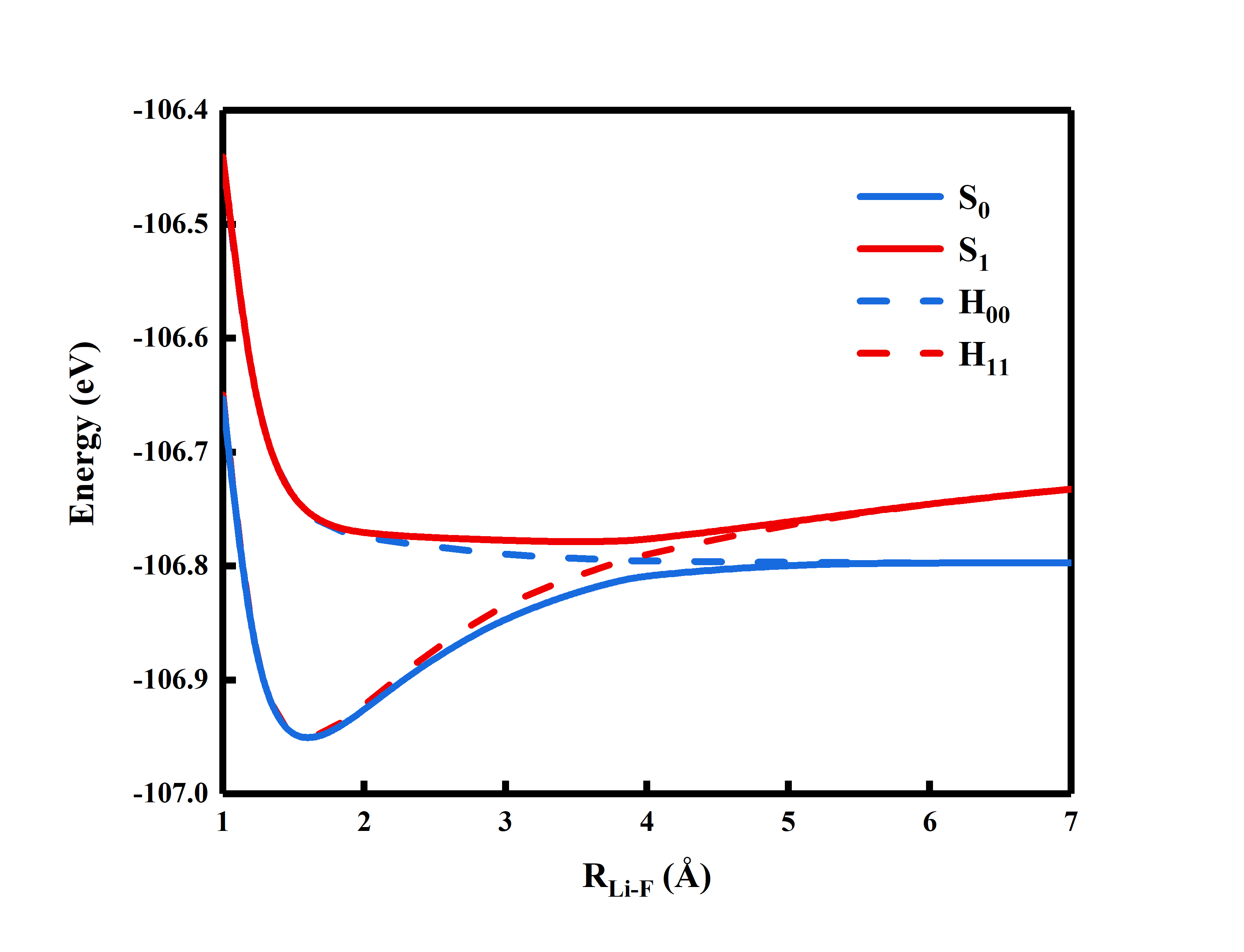
1.4.6. VBCAD Analysis of LiF Molecule
LiF VBCAD
$ctrl
vbscf
str=full nae=2 nao=2
iscf=5
int=libcint basis=aug-cc-pvtz
wstate(1)=1,1 vbcad itmax=500
$end
$actorb
1
2
$end
$geo
F    0.0 0.0  0.0
Li   0.0 0.0  3.8
$end
$gus
1 1
2 2
3 3
4 4
5 5
6 6
7 7
$end
Tip
By using the simplified input format, the
$ACTORBsection only required user to input the active orbitals.Users are encouraged to experiment with different bond lengths at RLi-F = 1.0, 1.2, 1.4, 1.6, 1,8, 2.0, 2.4, 2.6, 2.8, 3.0, 4.0, 7.0 Angstrom, get the energies and plot the potential energy surface. See at which distance the diabatic states cross. Following is the example of the potential energy surface.
To scan the potential energy surface, it is recommended that the user replace the content of
$GUSby the content of.orbfrom the points nearby.
1.4.7. Geometry Optimization of the Kekulé structure of benzene molecule
Kekule benzene Gopt
$ctrl
vbscf
nstr=1 nae=6 nao=6
iscf=5
int=libcint basis=cc-pvdz
itmax=500
opt
$end
$str
1:18 19 20 21 22 23 24
$end
$actorb
1
2
3
4
5
6
$end
$geo
C       0.000000     1.395000     0.000000
C       1.208000     0.697000     0.000000
C       1.208000    -0.697000     0.000000
C       0.000000    -1.395000     0.000000
C      -1.208000    -0.697000     0.000000
C      -1.208000     0.697000     0.000000
H       0.000000     2.495000     0.000000
H       2.161000     1.247000     0.000000
H       2.161000    -1.247000     0.000000
H       0.000000    -2.495000     0.000000
H      -2.160000    -1.247000     0.000000
H      -2.160000     1.247000     0.000000
$end
$gus
1   1
2   2
3   3
4   4
5   5
6   6
7   7
8   8
9   9
10  10
11  11
12  12
13  13
14  14
15  15
16  16
17  18
18  19
19  17
20  17
21  17
22  17
23  17
24  17
$end
1.4.8. Geometry Optimization of the Dewar structure of benzene molecule
Dewar benzene Gopt
$ctrl
vbscf
nstr=1 nae=6 nao=6
iscf=5
int=libcint basis=cc-pvdz
itmax=500
opt
$end
$str
1:18 19 20 21 24 22 23
$end
$actorb
1
2
3
4
5
6
$end
$geo
C       0.000000     1.395000     0.000000
C       1.208000     0.697000     0.000000
C       1.208000    -0.697000     0.000000
C       0.000000    -1.395000     0.000000
C      -1.208000    -0.697000     0.000000
C      -1.208000     0.697000     0.000000
H       0.000000     2.495000     0.000000
H       2.161000     1.247000     0.000000
H       2.161000    -1.247000     0.000000
H       0.000000    -2.495000     0.000000
H      -2.160000    -1.247000     0.000000
H      -2.160000     1.247000     0.000000
$end
$gus
1   1
2   2
3   3
4   4
5   5
6   6
7   7
8   8
9   9
10  10
11  11
12  12
13  13
14  14
15  15
16  16
17  18
18  19
19  17
20  17
21  17
22  17
23  17
24  17
$end
1.5. Theory and Methodologies
In this appendix, a brief introduction to VB theory and methodologies will be given to the users. For more detailed information, it is recommended to the users to read our reviews and research papers.
1.5.1. Introduction to VB Theory
In quantum chemistry, the many-electron wave function for a system is expressed as a linear combination of state functions:
In spin-free quantum chemistry, state functions \(\Phi_{K}\) should be a spin eigenfunction with anti-symmetry with respect to permutation of electron indices.The wave function is of the form
where \(\hat{A}\) is an antisymmetrizer, \(\Omega_0\) is an orbital product as
where \(\phi_i\) is the set of VB orbitals which can be purely localized hybrid atomic orbitals (HAOs), bond distorted orbitals (BDOs, delocalized along the bonding direction), and totally delocalized overlap enhanced orbitals (OEOs), and \(\Theta_{K}\) is a spin function. For VB methods, the state functions are VB functions, and their spin functions may be taken as the Rumer basis sets
where \(\left(ij\right)\) runs over all bonds and k over all unpaired electrons. Given an orbital product \(\Omega_0\) a complete set of VB functions is constructed by choosing all independent spin functions \(\Theta_{K}\) .
The coefficients \(C_{K}\) in Eq. (A.1) are determined by solving the conventional secular equation \(\mathbf{HC}=E\mathbf{MC}\) , where Hamiltonian and overlap matrices are defined as follows:
and
Structural weights are given by the Coulson-Chirgwin formula
Eqs. (A.5) and (A.6) involve N! terms due to antisymmetrizer \(\hat{A}\) . If one-electron functions are orthogonal, only a few terms are non-zero and make contributions to the matrix elements, and consequently the matrix elements can be conveniently evaluated. However, in VB methods, non-orthogonal orbitals are generally used, and thus all N! terms make contributions to the matrix elements. Although it is not necessary to expand all N! terms to evaluate a determinant, the computational demanding in VB calculations is in general much more than that in MO calculations.
1.5.2. The Evaluation of Hamiltonian and Overlap Matrices
In the XMVB package, two algorithms are implemented to compute the Hamiltonian and overlap matrices: one based on the Slater determinant expansion method, and the other based on the paired-permanent-determinant method.
1.5.2.1. Slater determinant expansion algorithm
Traditionally, an HLSP function is expressed in terms of \(2^{m}\) Slater determinants (m is the number of covalent bonds of structure),
where \(D(\Omega_K)\) is a Slater determinant corresponding to Eq. (A.3), \(P_{i}\) is an operator that exchanges the spins of the two electrons forming the i-th bond.
Example: An HLSP function corresponding to a Kekulé structure of benzene is written as
The Hamiltonian matrix element is expressed as
where \(f_{rs}\) and \(g_{rs,ut}\) are one-electron and two-electron integrals respectively, and \(D(S_r^s)\) and \(D(S_{ru}^{st})\) are the first and the second order cofactors of the overlap matrix between the two determinants respectively. Cofactors are computed by the Jacobi ratio theorem. The costs are of the order \(N^3\) for the first order and \(N^4\) for the second order cofactors at most.
1.5.2.2. Paired-permanent-determinant approach
Paired-permanent-determinant (PPD) approach is based on the spin-free form of VB theory. In the spin-free VB theory, the Hamiltonian and overlap matrix elements are now written as
and
respectively, where is the first diagonal element of the standard irreducible representation of permutation P of the symmetric group \(S_{N}\). In the PPD approach, a function, called PPD, is defined as follow:
Given an N × N square matrix
the PPD of \(\mathbf{A}\) for the irreducible representation \([ \lambda ]\) is the number
The evaluation of a PPD function is performed by a procedure similar to the Laplacian expansion algorithm for determinant. Hamiltonian and overlap matrix elements are computed by multiplying electronic integrals with their corresponding cofactors of PPDs. Evaluation of a PPD is more complicated than that of a determinant. But it can be beneficial when there are many bonded pairs in system. In that case there are only a few PPDs rather than numerous determinants to be evaluated.
1.5.3. Orbital Optimization
The gradient vectors of energy are evaluated in four ways: the first is the numerical approximation by differential method; the second is analytical gradient based on Fock matrices, using only the first order density matrix; the third is analytical based on the first and the second order orbital density matrices; and the third is based on generalized Brillouin theorem. The first three methods are fitted for all-type orbitals, and the later one is only available for strictly localized and delocalized orbitals. The second one is suitable only when there is no orthogonality between VB functions. There are two orbital optimization methods adopted in the package. The optimization with numerical gradient is based on the Davidson-Fletcher-Powell (DFP) family of variable metric methods, and the optimization with analytical gradient is proceeded with limited-memory Broyden-Fletcher-Goldfarb-Shanno (L-BFGS) method.
1.5.4. The VBSCF Methods
The wave function of Valence Bond Self Consistent Field (VBSCF) method is the linear combination of VB structures, as shown in eq.(A.1). In VBSCF method, All VB structures share the same set of VB orbitals, and both sets of the structure coefficients and VB orbitals are optimized simultaneously to minimize the total energy. This is comparable to the MCSCF method in the MO theory. VBSCF method takes care of the static electron correlation and gives equivalent results to the MO-based CASSCF calculations. It should be noted that the dynamic electron correlation is not accounted for in the VBSCF method. In XMVB, VBSCF method is the default method, thus this keyword can be ignored.
1.5.5. Post-VBSCF Method
The VBSCF result includes only static correlation energy, which makes VBSCF results not accurate enough for quantitative researches. The purpose of post-VBSCF methods is to take dynamic correlation into account as much as possible to get accurate enough results. There are several post-VBSCF methods developed so far and will be introduced in this section. It is strongly recommended to perform post-VBSCF calculations with initial guesses from a pre-proceeded VBSCF calculation. As to VBCI and VBPT2, this is enforced.
1.5.5.1. The BOVB Method
The orbitals of Breathing Orbital Valence Bond (BOVB) method are also optimized by SCF procedure, as VBSCF does. The difference between VBSCF and BOVB methods is that BOVB provides an extra degree of freedom during orbital optimization. In BOVB method, each VB structure has its own set of orbitals and are optimized independently
Thus, the orbitals adopt themselves to the instantaneous field of the VB structures, rather than to the mean field of all the structures in VBSCF. This degree of freedom makes the orbitals in BOVB “breathing” in different structures, introduces dynamic correlation, and thereby improves considerably the accuracy of VB computations.
1.5.5.2. The VBCI Method
The VBCI method is based on localized VB orbitals. In this method VB orbitals are divided to several blocks (occupied and virtual orbitals). Excited VB structures are generated by replacing occupied VB orbitals with virtual orbitals that are localized on the same block. The wave function of VBCI is the linear combination of all reference and excited VB structures
where \(\Phi^i_K\) is CI structure coming from VBSCF structure K, including reference and excited structures, and the coefficients \({C_{Ki}}\) are obtained by solving the secular equation. The VBCI weight can be given either with eq. (A.7), which gives weights of all CI structures, or in a more compact way as
where \(W_K\) is the contracted weights of reference structure K, including weights of all CI structures coming from structure K.
Allowing for different excitations for different electronic shells, currently the VBCI method consists of the following calculation levels:
VBCI(S,S): only single excitations are involved in either active electron or inactive electron. In brief, this is a VBCIS procedure.
VBCI(D,S): the active shell is treated by single and double excitations, whereas the inactive shell by single excitations only. Also included in this level are double excitations which consist of a single excitation from each shell.
VBCI(D,D): single and double excitations are involved for both active and inactive electrons, in short, VBCISD.
1.5.5.3. The VBPT2 Method
Another post-VBSCF method is Valence Bond second-order Perturbation Theory (VBPT2) method. The wave function of VBPT2 can be separated into 2 parts as
where VBSCF wave function is taken as the zeroth-order wave function \(\Psi^0\), and the first-order part is the combination of singly and doubly excited wave functions
To enhance the efficiency of VBPT2, the virtual orbitals are delocalized and orthogonal to the occupied space, and the excitations include all virtual orbitals. In this manner, the excited structures in VBPT2 don’t belong to any fundamental structure, and the matrix elements can be calculated easily with Coulson-Slater rules.
1.5.5.4. The DFVB Method
Density functional valence bond (DFVB) method is a VB computational method which combines VBSCF and DFT correlation functional. In DFVB method, the wave function, density and static correlation energy is provided by VBSCF method, while the dynamic correlation energy is obtained by DFT correlation functional. The total energy formalism of DFVB is expressed as:
where \(E^\textrm{VBSCF}\) is the VBSCF part, including static correlation energy, and \(E_\textrm{C}\left[\rho^\textrm{VB}\right]\) is the DFT correlation energy obtained by a functional according to current VB density \(\rho^\textrm{VB}\) . The total energy and wave function is optimized through a SCF procedure. In practice, GGA correlation functionals, such as LYP, PW, PBE correlation functional, are recommended functionals.
1.5.6. Solvation VB Methods
1.5.6.1. The VBPCM Method
The VBPCM method is an ab initio solvation VB method that is based on implicit solvation model PCM in which the state wave function is expressed in the usual terms as a linear combination of VB structures. The Schrödinger equation of VBPCM is expressed as
where \(\hat{H}^0\) is the Hamiltonian operator in vacuum and \(\hat{V}^{\textrm{PCM}}\) is the solvation potential obtained by PCM. The VBPCM wave function and energy are optimized simultaneously in an SCF procedure. VBPCM is now available for VBSCF and BOVB.
VBPCM has been used in several researches. VBPCM has been rewritten in XMVB 2.0 and is capable for hetero-PCM and EFP/PCM calculations.
1.5.6.2. The VBEFP Method
The VBEFP method is an QM/MM method in which the QM part is expressed as a VB wave function and the MM part is expressed with EFP1, which is a polarized water model proposed by Gordon et al. The VBEFP energy is obtained by following equation
where \(\hat{H}^0\) is the Hamiltonian operator in vacuum and \(\hat{V}^{\textrm{EFP}}\) is the solvation potential obtained by EFP method. An SCF procedure is used to optimize the wave function and energy of VBEFP simultaneously.
Currently, VBEFP is available only in module distribution and is only available for VBSCF. With the use of EFP, VBEFP is very useful to take strong and short solvent-solute interactions into account.
2. Tutorial
2.1. BDE and RE of F2
2.1.1. Introduction
F2 is a typical diatimic molecule which is simple enough for the users as a starting point. There is only 1 chemical bonding in the molecule. The 3 structures of the bonding is shown below.
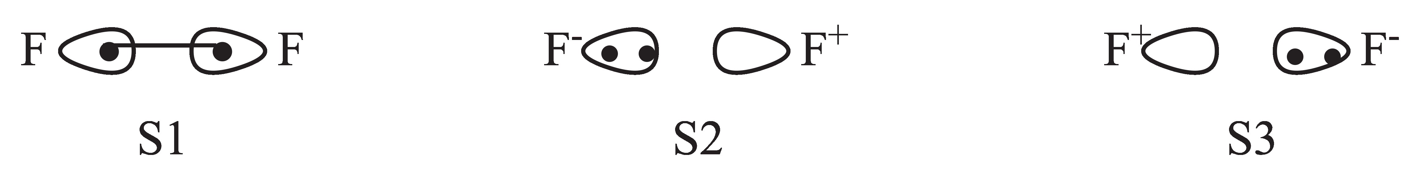
Fig. 2.1.1 Structures of F2 molecule
Here S1 denotes the covalent structure in which two active electrons are shared between both F atoms while S2 and
S3 denote 2 quivalent ionic structures in which two active eletrons doubly occupy orbital on certain F atom.
In this exercise, we will try to proceed computations for the bond dissociation energy (BDE) and resnance energy (RE) of F2. This takes computations at stationary point and dissociation limit with various sets of VB structures. This exercise will provide a first glance at VB computation. The users will learn the struct and syntax of XMVB input, how to build a simple input file, how to run the job and what we will get from the output.
Note
This exercise just shows the users how to proceed a VBSCF computation for a specific molecule, what we can get from the output and how to analyze the results. The accurate computation of BDE of F2 requires higher level computational methods with delocalized inactive \(\pi\) orbitals.
2.1.2. Computations with 3 Structures at Stationary Point
The computations are proceeded with F-F bond length 1.4 Angstrom, and the basis set is cc-pVDZ. For simplicity, F atoms are located in the Z axis.
2.1.2.1. Input File
Here shows the XMVB input file for all 3 structures at stationary point:
F2 VBSCF with 3 structures
$CTRL
VBSCF
STR=FULL NAO=2 NAE=2 ISCF=5
ORBTYP=HAO FRGTYP=SAO
INT=LIBCINT BASIS=CC-PVDZ
$END
$FRAG
1*6
SPZDXXDYYDZZ 1
SPZDXXDYYDZZ 2
PXDXZ 1
PXDXZ 2
PYDYZ 1
PYDYZ 2
$END
$ORB
1*10
1
2
1
2
3
4
5
6
1
2
$END
$GEO
F 0.0 0.0 0.0
F 0.0 0.0 1.4
$END
The global keywords listed in $CTRL section are explained below:
STR=FULLXMVB generates all VB structures automatically according to a specific active space.ISCF=5VBSCF computation with RDM-based algorithm.IPRINT=3XMVB will print most information.NAO=2andNAE=2Specify the active space with 2 active orbital and 2 active electrons respectively.ORBTYP=HAOandFRGTYP=SAOThe VB orbitals are described with fragments.INT=LIBCINTIntegrals are evaluated by XMVB withLIBCINTlibrary.BASIS=CC-PVDZThe basis set is cc-pVDZ.
Note
The orbitals of a molecule can be devided into “inactive” and “active” parts. The inactive orbitals are always doubly occupied in all VB structures, while the occupation numbers of active orbitals can be 0, 1 or 2 in each VB structure.
$FRAG section describes the fragments used to construct VB orbitals. In this case, the first line 1*6 means that there are 6 fragments built and each fragment include only 1 atom. The details of fragments are described in the following lines. For example, SPZDXXDYYDZZ 1 means that the fragment includes s, pz, dxx, dyy and dzz basis functions on atom 1, which is the first F atom in this case.
$ORB section describes VB orbitals. The first line 1*10 means that there are 10 orbitals in this case, each consisting of only 1 fragment. Each line below describes one orbital. For example, the first orbital includes only fragment 1, meaning that this orbital locates on the first F atom and belongs to the \(\sigma\) space since the F-F lies on Z axis. Also, orbital 6 with fragment 4 shows that the orbital describes the \(\pi_x\) orbital on the first F atom.
$GEO section shows the geometry of F2 molecule. Both Cartesian and internal coordinates are supported.
Note
Since NAO=2 is specified in $CTRL section, the last 2 orbitals in $ORB should be the active orbitals.
It is highly recommended that active orbitals are always palced after the inactive ones. This may make the input file more readable and less possible to get error.
2.1.2.2. Computational Results
In this case, 3 VB structures are generated with 1 covalent structure (0th ion structure) and 2 ionic structures (1th ion structures). These structures can be expaned into 4 determinants.
Number of   0th ion  structures  is:          1  from          1 to          1
Number of   0th ion determinants is:          2  from          1 to          2
Number of   1th ion  structures  is:          2  from          2 to          3
Number of   1th ion determinants is:          2  from          3 to          4
Total number of  structures  is:          3
Total number of determinants is:          4
                   .
                   .
                   .
Number of Structures:           3

The following structures are used in calculation:

      1 *****  1:8    9  10
      2 *****  1:8    9   9
      3 *****  1:8   10  10
The user may find from the output file that the VBSCF converged after 25 iterations and the final energy is -198.75115493 hartree.
                       VBSCF converged in    25 iterations

Total Energy:    -198.75115493

First Excited:   -197.880879
The coefficients and weights shows the importance of each structure. Following are the coefficients and weights of generated VB structures. Both coefficients and weights show that the covalent structure is the dominant one. So the F-F bond should be a covalent bond.
       ******  COEFFICIENTS OF STRUCTURES ******

1    -0.80579  ******  1:8    9  10
2    -0.21326  ******  1:8    9   9
3    -0.21326  ******  1:8   10  10
                  .
                  .
                  .
       ******  WEIGHTS OF STRUCTURES ******

1     0.77586  ******  1:8    9  10
2     0.11207  ******  1:8    9   9
3     0.11207  ******  1:8   10  10
Finally, the bond order value (0.773) in atomic population analysis shows that F-F bond should be a single bond.
          ******  BOND ORDER  ******

ATOM 1        ATOM 2           DIST     BOND ORDER

 1 F           2 F            1.400       0.773
2.1.3. Computations with 3 Structures at Dissociation Limit
2.1.3.1. Input File
The input file for such computation can be easily obtained by modifying the corresponding one at stationary point. As shown below, one just needs to modify the coordinate of the second F atom to change 1.4 to 10.0. This will increase the F-F bond distance to 10.0 Angstrom.
$GEO
F 0.0 0.0 0.0
F 0.0 0.0 10.0
$END
2.1.3.2. Computational Results
After SCF procedure, the user will get the final energy as shown below. The computational energy of dissociated F2 is -198.74386524 hartree.
Total Energy:    -198.74386524

First Excited:   -197.850852
Both coefficients and weights of VB structures show that the wave function includes only covalent structure, indicating that the molecule is dissociated to 2 F\(\cdot\) radicals.
       ******  COEFFICIENTS OF STRUCTURES ******

1     1.00000  ******  1:8    9  10
2     0.00000  ******  1:8    9   9
3     0.00000  ******  1:8   10  10
                      .
                      .
                      .
       ******  WEIGHTS OF STRUCTURES ******

1     1.00000  ******  1:8    9  10
2     0.00000  ******  1:8    9   9
3     0.00000  ******  1:8   10  10
By substracting energies at stationary point and dissociation limit, the BDE can be obtained as 4.4 kcal/mol.
2.1.4. Computations with Covalent Structure at Stationary Point
2.1.4.1. Input File
The input file can be obtained by replacing STR=FULL with STR=COV in the input file of 3 structures at stationary point, as shown below.
$CTRL
VBSCF
STR=COV NAO=2 NAE=2 ISCF=5
ORBTYP=HAO FRGTYP=SAO
INT=LIBCINT BASIS=CC-PVDZ
$END
2.1.4.2. Computational Results
The structure information is shown below. It can be seen that only 1 covalent structure is generated for this computation.
Number of   0th ion  structures  is:          1  from          1 to          1
Number of   0th ion determinants is:          2  from          1 to          2
Total number of  structures  is:          1
Total number of determinants is:          2
                       .
                       .
                       .
 Number of Structures:           1

 The following structures are used in calculation:

       1 *****  1:8    9  10
The final energy after SCF iteration is -198.67485969 hartree.
Total Energy:    -198.67485969

The Last Change in Energy:  -0.000000
The bond order result in atomic population analysis shows that the bond order with only covalent structure is 0.324, which is much smaller than computations with 3 structures.
          ******  BOND ORDER  ******

ATOM 1        ATOM 2           DIST     BOND ORDER

 1 F           2 F            1.400       0.324
The RE value, 47.6 kcal/mol, can be obtained from energies by covalent and 3 structure computations at stationary point. Compared with the computational BDE 4.4, RE is much larger than BDE, indicating that the chemical bonding in F2 is an charge-shifting bond. The much smaller bond order data with only covalent structure also indicates that resonance plays an important role in the F-F bonding.
2.2. Resonance in C6H6
2.2.1. Introduction
Benzene (C6H6) is a classical aromatic molecule in which electrons in \(\pi\) space are delocalized. The covalent valence bond structures are shown in the following table.
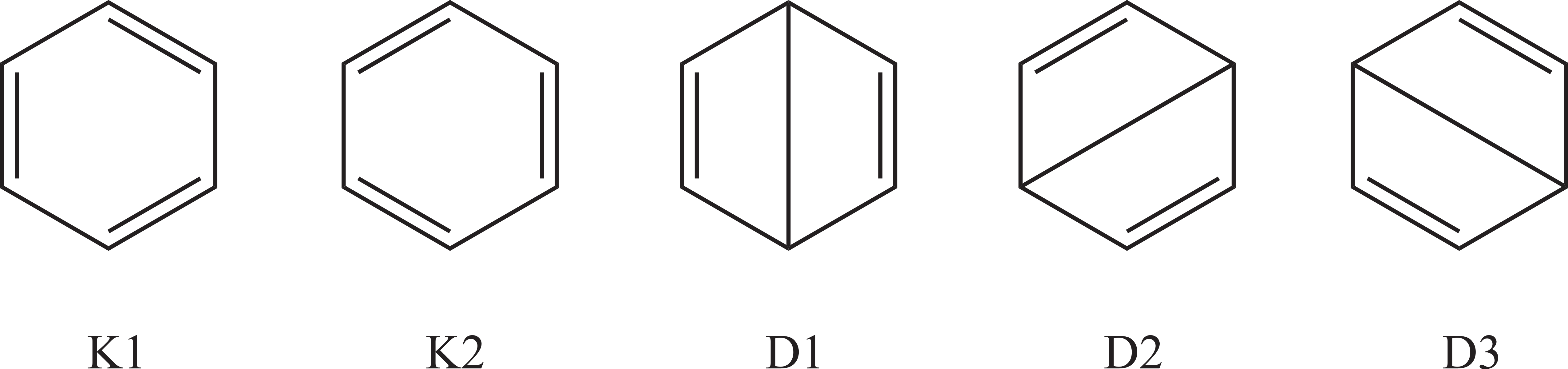
Fig. 2.2.1 Covalent Structures of C6H6
The 5 covalent structures can be classified as 2 types: the first 2 structures are Kekulé structures and the others are regarded as Dewar structures. In this exercise, the resonance energy in the benzene molecule will be computed to show how resonance stabilize the aromatic molecule.
2.2.2. Computations with 5 Covalent Structures
First, we will compute the energy with all 5 covalent structures.
2.2.2.1. Input File
The input file is shown below.
C6H6
$ctrl
vbscf
str=cov nao=6 nae=6 iscf=5
orbtyp=hao frgtyp=sao
int=libcint basis=cc-pvdz
$end
$frag
12 2*6
spxpydxxdyydzzdxy 1-12
pzdxzdyz 1 2
pzdxzdyz 3 4
pzdxzdyz 5 6
pzdxzdyz 7 8
pzdxzdyz 9 10
pzdxzdyz 11 12
$end
$orb
1*18 1*6
1
1
1
1
1
1
1
1
1
1
1
1
1
1
1
1
1
1
2
3
4
5
6
7
$end
$geo
 C           0.6995000584   1.2115696411   0.0000000000
 H           1.2460106991   2.1581538376   0.0000000000
 C          -0.6995000584   1.2115696411   0.0000000000
 H          -1.2460106991   2.1581538376   0.0000000000
 C          -1.3990001169   0.0000000000   0.0000000000
 H          -2.4920213982   0.0000000000   0.0000000000
 C          -0.6995000584  -1.2115696411   0.0000000000
 H          -1.2460106991  -2.1581538376   0.0000000000
 C           0.6995000584  -1.2115696411   0.0000000000
 H           1.2460106991  -2.1581538376   0.0000000000
 C           1.3990001169   0.0000000000   0.0000000000
 H           2.4920213982   0.0000000000   0.0000000000
$end
In this input file, the molecule lays in the XY plane. The fragments specified in $FRAG section are defined according to the symmetries. Since we concern on the resonance in \(\pi\)space, electrons locating in \(\sigma\)space is not in the interest. Thus eletrons in the \(\sigma\)orbitals can be treated as inactive ones and make them delocalized in all structures. To this reason, the first fragment is defined to include all basis functions in \(\sigma\) space in the molecule. The remained fragments denote \(\pi\) orbitals locates on each CH group.
2.2.2.2. Computational Results
5 VB structures will be generated in the computation and can be found in the output:
Number of Structures:           5

The following structures are used in calculation:

      1 *****  1:18  21  22  20  23  19  24
      2 *****  1:18  20  21  22  23  19  24
      3 *****  1:18  20  21  19  22  23  24
      4 *****  1:18  19  20  22  23  21  24
      5 *****  1:18  19  20  21  22  23  24
Final energy can be found after the VBSCF iteration as -230.63450 hartree.
Total Energy: -230.63449533
Both coefficients and weights of VB structures show that structures are in 2 groups. Structure 2 and 5 correspond to the Kekulé structures, which are the dominant ones, and the others denote Dewar structures.
       ******  COEFFICIENTS OF STRUCTURES ******

1     0.14537  ******  1:18  21  22  20  23  19  24
2    -0.40098  ******  1:18  20  21  22  23  19  24
3     0.14537  ******  1:18  20  21  19  22  23  24
4     0.14537  ******  1:18  19  20  22  23  21  24
5    -0.40098  ******  1:18  19  20  21  22  23  24
       ******  WEIGHTS OF STRUCTURES ******

1     0.11245  ******  1:18  21  22  20  23  19  24
2     0.33132  ******  1:18  20  21  22  23  19  24
3     0.11245  ******  1:18  20  21  19  22  23  24
4     0.11245  ******  1:18  19  20  22  23  21  24
5     0.33132  ******  1:18  19  20  21  22  23  24
The atomic population analysis shows that the bond orders of all CC bondings are the same as 1.188, showing the effect of conjugation.
          ******  BOND ORDER  ******

ATOM 1        ATOM 2           DIST     BOND ORDER

 1 C           2 H            1.093       0.979
 1 C           3 C            1.399       1.188
 3 C           4 H            1.093       0.979
 3 C           5 C            1.399       1.188
 5 C           6 H            1.093       0.979
 5 C           7 C            1.399       1.188
 7 C           8 H            1.093       0.979
 7 C           9 C            1.399       1.188
 9 C          10 H            1.093       0.979
 1 C          11 C            1.399       1.188
 9 C          11 C            1.399       1.188
11 C          12 H            1.093       0.979
2.2.3. Computations with 2 Kekulé Structures
2.2.3.1. Input File
The input file is shown below.
C6H6
$ctrl
vbscf
nstr=2 nao=6 nae=6 iscf=5
orbtyp=hao frgtyp=sao
int=libcint basis=cc-pvdz
guess=read
$end
$str
1:18 19-24
1:18 19 24 20 21 22 23
$end
$frag
12 2*6
spxpydxxdyydzzdxy 1-12
pzdxzdyz 1 2
pzdxzdyz 3 4
pzdxzdyz 5 6
pzdxzdyz 7 8
pzdxzdyz 9 10
pzdxzdyz 11 12
$end
$orb
1*18 1*6
1
1
1
1
1
1
1
1
1
1
1
1
1
1
1
1
1
1
2
3
4
5
6
7
$end
$geo
C 0.6995000584 1.2115696411 0.0000000000
H 1.2460106991 2.1581538376 0.0000000000
C -0.6995000584 1.2115696411 0.0000000000
H -1.2460106991 2.1581538376 0.0000000000
C -1.3990001169 0.0000000000 0.0000000000
H -2.4920213982 0.0000000000 0.0000000000
C -0.6995000584 -1.2115696411 0.0000000000
H -1.2460106991 -2.1581538376 0.0000000000
C 0.6995000584 -1.2115696411 0.0000000000
H 1.2460106991 -2.1581538376 0.0000000000
C 1.3990001169 0.0000000000 0.0000000000
H 2.4920213982 0.0000000000 0.0000000000
$end
$gus
90 90 90 90 90 90 90 90 90 90 90 90 90 90 90 90 90 90 5 5 5 5 5 5
# ORBITAL 1 NAO = 90
-0.4085807072 1 -0.0018715270 2 0.0001649808 3 0.0000999746 4
0.0001985368 5 0.0000470242 7 0.0000880828 8 0.0009574571 10
0.0000833088 11 0.0010378240 13 0.0011389938 15 -0.0001957425 16
-0.0001334195 17 0.0000477351 18 0.0000812855 19 -0.4085807076 21
-0.0018715190 22 0.0001649828 23 -0.0000999676 24 0.0001985300 25
-0.0000470232 27 0.0000880811 28 0.0009574481 30 -0.0000833266 31
0.0010378340 33 0.0011390026 35 -0.0001957414 36 -0.0001334204 37
-0.0000477371 38 0.0000812776 39 -0.4090845359 41 -0.0018966521 42
0.0001488619 43 -0.0002148556 44 0.0000001381 45 -0.0000988751 47
0.0000000169 48 0.0010810968 50 -0.0000001656 51 0.0009153322 53
0.0011399821 55 -0.0002143575 56 -0.0001372115 57 -0.0000966788 58
0.0000001529 59 -0.4085807085 61 -0.0018714717 62 0.0001649779 63
-0.0001000242 64 -0.0001983775 65 -0.0000470512 67 -0.0000879863 68
0.0009574723 70 0.0000839012 71 0.0010378364 73 0.0011390336 75
-0.0001956328 76 -0.0001334448 77 -0.0000479296 78 -0.0000811013 79
-0.4085807082 81 -0.0018714747 82 0.0001649755 83 0.0001000278 84
-0.0001983820 85 0.0000470479 87 -0.0000879885 88 0.0009574749 90
-0.0000838796 91 0.0010378346 93 0.0011390280 95 -0.0001956337 96
-0.0001334457 97 0.0000479178 98 -0.0000811144 99 -0.4090845352 101
-0.0018966413 102 0.0001488609 103 0.0002148576 104 0.0000001396 105
0.0000988788 107 0.0000000209 108 0.0010810705 110 0.0000001777 111
0.0009153543 113 0.0011399863 115 -0.0002143672 116 -0.0001372134 117
0.0000966809 118 0.0000001629 119
# ORBITAL 2 NAO = 90
0.2888930861 1 0.0012304770 2 -0.0002563966 3 0.0001336859 4
-0.0001561191 5 0.0001914831 7 -0.0001481897 8 -0.0008221343 10
-0.0001557600 11 -0.0005906595 13 -0.0007980351 15 0.0001543642 16
0.0000791296 17 0.0000125324 18 -0.0000788689 19 -0.2888931497 21
-0.0012304753 22 0.0002562013 23 0.0001337942 24 0.0001566737 25
0.0001915140 27 0.0001494777 28 0.0008219804 30 -0.0001516843 31
0.0005907316 33 0.0007979421 35 -0.0001550608 36 -0.0000790540 37
0.0000136909 38 0.0000800072 39 -0.5781904466 41 -0.0024581181 42
0.0005050109 43 -0.0001390292 44 0.0000000205 45 -0.0000746810 47
0.0000000140 48 0.0015287631 50 -0.0000000553 51 0.0012982685 53
0.0015971801 55 -0.0003048222 56 -0.0001585226 57 -0.0001238936 58
0.0000000479 59 -0.2888930865 61 -0.0012304541 62 0.0002561993 63
0.0001337970 64 -0.0001566499 65 0.0001915245 67 -0.0001494674 68
0.0008219645 70 0.0001517465 71 0.0005907569 73 0.0007979557 75
-0.0001550484 76 -0.0000790645 77 0.0000136980 78 -0.0000799949 79
0.2888931500 81 0.0012304673 82 -0.0002563957 83 0.0001337007 84
0.0001561303 85 0.0001914997 87 0.0001482011 88 -0.0008221145 90
0.0001556889 91 -0.0005906834 93 -0.0007980414 95 0.0001543768 96
0.0000791346 97 0.0000125801 98 0.0000788956 99 0.5781904449 101
0.0024591332 102 -0.0005052562 103 -0.0001393968 104 0.0000000109 105
-0.0000739491 107 -0.0000000104 108 -0.0015297884 110 -0.0000000183 111
-0.0012968826 113 -0.0015966043 115 0.0003041670 116 0.0001581403 117
-0.0001241023 118 -0.0000000148 119
# ORBITAL 3 NAO = 90
0.5006118878 1 0.0021171792 2 -0.0004445363 3 -0.0001718795 4
-0.0000528411 5 -0.0001543791 7 0.0000142568 8 -0.0010905424 10
-0.0000444470 11 -0.0013582539 13 -0.0013824483 15 0.0002505625 16
0.0001341232 17 -0.0000778672 18 -0.0000745639 19 0.5006118515 21
0.0021171388 22 -0.0004445339 23 0.0001718621 24 -0.0000528197 25
0.0001543481 27 0.0000142554 28 -0.0010905019 30 0.0000444391 31
-0.0013583104 33 -0.0013824752 35 0.0002505629 36 0.0001341408 37
0.0000778110 38 -0.0000745770 39 -0.0000000362 41 0.0000000221 42
-0.0000000048 43 0.0000000087 44 0.0002083308 45 -0.0000000157 47
0.0002704667 48 -0.0000000212 50 0.0002206198 51 0.0000000294 53
0.0000000132 55 -0.0000000141 56 -0.0000000081 57 0.0000000045 58
0.0000602462 59 -0.5006118875 61 -0.0021171392 62 0.0004445257 63
-0.0001718574 64 -0.0000528443 65 -0.0001543471 67 0.0000142010 68
0.0010904959 70 0.0000442655 71 0.0013583140 73 0.0013824713 75
-0.0002505931 76 -0.0001341382 77 -0.0000777637 78 -0.0000746227 79
-0.5006118506 81 -0.0021171793 82 0.0004445278 83 0.0001718746 84
-0.0000528666 85 0.0001543776 87 0.0000142018 88 0.0010905358 90
-0.0000442668 91 0.0013582572 93 0.0013824439 95 -0.0002505929 96
-0.0001341203 97 0.0000778157 98 -0.0000746149 99 0.0000000372 101
0.0000000233 102 -0.0000000051 103 -0.0000000081 104 0.0002082947 105
0.0000000157 107 0.0002704090 108 -0.0000000235 110 -0.0002208132 111
0.0000000315 113 0.0000000132 115 -0.0000000150 116 -0.0000000085 117
-0.0000000048 118 0.0000600832 119
# ORBITAL 4 NAO = 90
-0.2891567875 1 -0.0011788380 2 0.0006696401 3 0.0001162136 4
-0.0000434029 5 0.0000569096 7 -0.0002181218 8 0.0005581052 10
-0.0000173221 11 0.0007001594 13 0.0007639834 15 -0.0000761592 16
-0.0000306619 17 0.0000222375 18 0.0000003327 19 -0.2891568478 21
-0.0011788552 22 0.0006696375 23 -0.0001162265 24 -0.0000433901 25
-0.0000569145 27 -0.0002181183 28 0.0005581234 30 0.0000173582 31
0.0007001375 33 0.0007639670 35 -0.0000761610 36 -0.0000306572 37
-0.0000222376 38 0.0000003522 39 0.5781677329 41 0.0024208733 42
-0.0012969300 43 -0.0000049661 44 -0.0000000187 45 -0.0003380963 47
0.0000000028 48 -0.0013034129 50 0.0000000076 51 -0.0012070190 53
-0.0015287103 55 0.0002187599 56 0.0000735925 57 0.0000329236 58
-0.0000000083 59 -0.2891567879 61 -0.0011788549 62 0.0006696380 63
-0.0001162154 64 0.0000433692 65 -0.0000569033 67 0.0002181026 68
0.0005581117 70 -0.0000174532 71 0.0007001480 73 0.0007639674 75
-0.0000761793 76 -0.0000306569 77 -0.0000221958 78 -0.0000003814 79
-0.2891568468 81 -0.0011788535 82 0.0006696419 83 0.0001162088 84
0.0000433741 85 0.0000569103 87 0.0002181062 88 0.0005581088 90
0.0000174178 91 0.0007001487 93 0.0007639740 95 -0.0000761773 96
-0.0000306542 97 0.0000222162 98 -0.0000003606 99 0.5781677327 101
0.0024208558 102 -0.0012969285 103 0.0000049612 104 -0.0000000253 105
0.0003380902 107 -0.0000000083 108 -0.0013033682 110 -0.0000000436 111
-0.0012070582 113 -0.0015287170 115 0.0002187773 116 0.0000735959 117
-0.0000329255 118 -0.0000000388 119
# ORBITAL 5 NAO = 90
-0.5007497195 1 -0.0020926701 2 0.0011274729 3 -0.0000664898 4
0.0000686296 5 -0.0002263515 7 -0.0001918806 8 0.0011015128 10
0.0000674501 11 0.0010736729 13 0.0013237329 15 -0.0001590050 16
-0.0000498765 17 0.0000054571 18 0.0000298585 19 0.5007496847 21
0.0020926790 22 -0.0011275085 23 -0.0000664796 24 -0.0000685616 25
-0.0002263533 27 0.0001920864 28 -0.0011015340 30 0.0000680448 31
-0.0010736610 33 -0.0013237436 35 0.0001589047 36 0.0000498846 37
0.0000056242 38 -0.0000296943 39 0.0000000348 41 0.0000000890 42
-0.0000000212 43 0.0000000320 44 0.0001851945 45 -0.0000000646 47
0.0002002088 48 -0.0000000915 50 0.0000942443 51 0.0000001220 53
0.0000000504 55 -0.0000000578 56 -0.0000000328 57 0.0000000176 58
0.0000247770 59 -0.5007497199 61 -0.0020926786 62 0.0011274738 63
0.0000664970 64 -0.0000686556 65 0.0002263560 67 0.0001918646 68
0.0011015108 70 0.0000673487 71 0.0010736709 73 0.0013237272 75
-0.0001590238 76 -0.0000498723 77 -0.0000054290 78 -0.0000298875 79
0.5007496855 81 0.0020926723 82 -0.0011275078 83 0.0000664707 84
0.0000685365 85 0.0002263476 87 -0.0001921026 88 -0.0011015386 90
0.0000681438 91 -0.0010736605 93 -0.0013237484 95 0.0001588863 96
0.0000498882 97 -0.0000056552 98 0.0000296659 99 0.0000000336 101
0.0000000883 102 -0.0000000217 103 -0.0000000323 104 -0.0001852396 105
0.0000000644 107 -0.0002002133 108 -0.0000000900 110 0.0000941944 111
0.0000001203 113 0.0000000496 115 -0.0000000565 116 -0.0000000328 117
-0.0000000169 118 -0.0000248210 119
# ORBITAL 6 NAO = 90
0.4091251475 1 0.0018241997 2 -0.0036592202 3 0.0000020694 4
-0.0000011859 5 0.0007741716 7 0.0013387077 8 -0.0007515405 10
0.0000812994 11 -0.0006732113 13 -0.0009930082 15 -0.0000359553 16
-0.0002099914 17 0.0000257544 18 0.0000416529 19 -0.4091251464 21
-0.0018242229 22 0.0036594107 23 0.0000019865 24 0.0000007218 25
0.0007741606 27 -0.0013398977 28 0.0007516717 30 0.0000776616 31
0.0006731473 33 0.0009930840 35 0.0000365738 36 0.0002099303 37
0.0000247332 38 -0.0000426613 39 0.4088400900 41 0.0018185067 42
-0.0036610579 43 -0.0000000395 44 0.0000000662 45 -0.0015467853 47
0.0000000329 48 -0.0006312514 50 -0.0000001499 51 -0.0007924283 53
-0.0009926163 55 -0.0000380211 56 -0.0002097659 57 -0.0000506940 58
0.0000001297 59 -0.4091251455 61 -0.0018241642 62 0.0036594070 63
0.0000019879 64 -0.0000006481 65 0.0007741792 67 0.0013399307 68
0.0007516425 70 -0.0000774650 71 0.0006732027 73 0.0009931240 75
0.0000366093 76 0.0002099034 77 0.0000247197 78 0.0000427155 79
0.4091251465 81 0.0018241721 82 -0.0036592195 83 0.0000021021 84
0.0000012118 85 0.0007742169 87 -0.0013386734 88 -0.0007514874 90
-0.0000814990 91 -0.0006732734 93 -0.0009930272 95 -0.0000359181 96
-0.0002099801 97 0.0000258758 98 -0.0000415851 99 -0.4088400890 101
-0.0018194794 102 0.0036612935 103 0.0000003129 104 0.0000000252 105
-0.0015474894 107 -0.0000000271 108 0.0006322381 110 -0.0000000559 111
0.0007910987 113 0.0009920653 115 0.0000386489 116 0.0002101309 117
-0.0000504971 118 -0.0000000437 119
# ORBITAL 7 NAO = 90
-0.0107819418 1 0.1790782666 2 0.0924284475 3 -0.0318865151 4
-0.0553049355 5 -0.0062977525 7 -0.0109401070 8 0.0108331095 10
-0.0038054399 11 0.0070287849 13 -0.0063313721 15 0.0455977157 16
0.0036387887 17 -0.0036035054 18 -0.0062459698 19 -0.0107819418 21
0.1790782665 22 0.0924284475 23 0.0318865153 24 -0.0553049354 25
0.0062977526 27 -0.0109401069 28 0.0108331095 30 0.0038054400 31
0.0070287847 33 -0.0063313720 35 0.0455977157 36 0.0036387887 37
0.0036035054 38 -0.0062459697 39 -0.0107755990 41 0.1791237848 42
0.0924406313 43 0.0638465961 44 -0.0000000002 45 0.0126243430 47
0.0000000000 48 0.0051202404 50 0.0000000002 51 0.0127397005 53
-0.0063317099 55 0.0456056414 56 0.0036342774 57 0.0072116661 58
-0.0000000001 59 -0.0107819418 61 0.1790782665 62 0.0924284475 63
0.0318865153 64 0.0553049352 65 0.0062977526 67 0.0109401069 68
0.0108331095 70 -0.0038054405 71 0.0070287846 73 -0.0063313721 75
0.0455977156 76 0.0036387886 77 0.0036035055 78 0.0062459696 79
-0.0107819418 81 0.1790782665 82 0.0924284475 83 -0.0318865153 84
0.0553049354 85 -0.0062977525 87 0.0109401069 88 0.0108331095 90
0.0038054404 91 0.0070287849 93 -0.0063313722 95 0.0455977156 96
0.0036387887 97 -0.0036035055 98 0.0062459696 99 -0.0107755990 101
0.1791237842 102 0.0924406314 103 -0.0638465970 104 -0.0000000002 105
-0.0126243426 107 0.0000000000 108 0.0051202413 110 -0.0000000001 111
0.0127397007 113 -0.0063317099 115 0.0456056422 116 0.0036342781 117
-0.0072116650 118 -0.0000000001 119
# ORBITAL 8 NAO = 90
0.0080809826 1 -0.1247496483 2 -0.0702559576 3 -0.0784948406 4
0.0639689094 5 -0.0281707685 7 0.0270146479 8 0.0056247890 10
0.0119191820 11 -0.0144007347 13 0.0039111625 15 -0.0517266720 16
-0.0069585491 17 0.0014215117 18 0.0074905042 19 -0.0080809832 21
0.1247496564 22 0.0702559624 23 -0.0784948380 24 -0.0639689094 25
-0.0281707673 27 -0.0270146491 28 -0.0056247882 30 0.0119191787 31
0.0144007344 33 -0.0039111628 35 0.0517266760 36 0.0069585494 37
0.0014215110 38 -0.0074905056 39 -0.0161618860 41 0.2495029330 42
0.1404967375 43 0.0323045190 44 0.0000000022 45 0.0186150565 47
0.0000000009 48 0.0009097151 50 0.0000000004 51 0.0166398753 53
-0.0078227360 55 0.1034460314 56 0.0139150017 57 0.0143938231 58
0.0000000000 59 -0.0080809826 61 0.1247496481 62 0.0702559577 63
-0.0784948405 64 0.0639689095 65 -0.0281707683 67 0.0270146490 68
-0.0056247889 70 -0.0119191785 71 0.0144007345 73 -0.0039111625 75
0.0517266726 76 0.0069585489 77 0.0014215107 78 0.0074905052 79
0.0080809832 81 -0.1247496565 82 -0.0702559623 83 -0.0784948381 84
-0.0639689091 85 -0.0281707675 87 -0.0270146480 88 0.0056247883 90
-0.0119191823 91 -0.0144007346 93 0.0039111629 95 -0.0517266754 96
-0.0069585496 97 0.0014215120 98 -0.0074905046 99 0.0161618860 101
-0.2495029327 102 -0.1404967374 103 0.0323045205 104 0.0000000024 105
0.0186150551 107 0.0000000008 108 -0.0009097149 110 -0.0000000002 111
-0.0166398772 113 0.0078227354 115 -0.1034460320 116 -0.0139150025 117
0.0143938213 118 0.0000000001 119
# ORBITAL 9 NAO = 90
0.0139974362 1 -0.2160783634 2 -0.1216786927 3 0.0639676065 4
-0.0045967336 5 0.0270145605 7 0.0030327889 8 -0.0179215924 10
0.0022068301 11 0.0027201810 13 0.0067737890 15 -0.0895686954 16
-0.0120431588 17 0.0074907427 18 0.0100672464 19 0.0139974359 21
-0.2160783579 22 -0.1216786897 23 -0.0639676097 24 -0.0045967367 25
-0.0270145618 27 0.0030327877 28 -0.0179215926 30 -0.0022068299 31
0.0027201819 33 0.0067737894 35 -0.0895686936 36 -0.0120431585 37
-0.0074907427 38 0.0100672457 39 -0.0000000003 41 0.0000000048 42
0.0000000027 43 0.0000000006 44 -0.1154605477 45 0.0000000003 47
-0.0437801763 48 0.0000000000 50 -0.0184419859 51 0.0000000003 53
-0.0000000002 55 0.0000000020 56 0.0000000003 57 0.0000000003 58
-0.0029035178 59 -0.0139974362 61 0.2160783627 62 0.1216786924 63
0.0639676067 64 -0.0045967344 65 0.0270145607 67 0.0030327888 68
0.0179215924 70 -0.0022068304 71 -0.0027201814 73 -0.0067737896 75
0.0895686955 76 0.0120431587 77 0.0074907427 78 0.0100672461 79
-0.0139974359 81 0.2160783587 82 0.1216786899 83 -0.0639676095 84
-0.0045967361 85 -0.0270145616 87 0.0030327879 88 0.0179215927 90
0.0022068297 91 -0.0027201816 93 -0.0067737889 95 0.0895686934 96
0.0120431584 97 -0.0074907426 98 0.0100672461 99 0.0000000003 101
-0.0000000048 102 -0.0000000027 103 0.0000000006 104 -0.1154605457 105
0.0000000004 107 -0.0437801767 108 -0.0000000001 110 0.0184419877 111
-0.0000000003 113 0.0000000001 115 -0.0000000020 116 -0.0000000003 117
0.0000000003 118 -0.0029035175 119
# ORBITAL 10 NAO = 90
-0.0051440589 1 0.1005718952 2 0.0845638529 3 -0.1397337895 4
0.1141834782 5 -0.0457303867 7 0.0234939964 8 0.0117656669 10
0.0056709072 11 -0.0100493795 13 -0.0019026433 15 0.0770087430 16
0.0164532289 17 -0.0072726819 18 -0.0060307741 19 -0.0051440587 21
0.1005718915 22 0.0845638499 23 0.1397337914 24 0.1141834780 25
0.0457303869 27 0.0234939969 28 0.0117656673 30 -0.0056709071 31
-0.0100493799 33 -0.0019026433 35 0.0770087402 36 0.0164532285 37
0.0072726816 38 -0.0060307738 39 0.0102806964 41 -0.2012853772 42
-0.1692333678 43 0.0582639973 44 -0.0000000022 45 -0.0049551221 47
-0.0000000006 48 0.0006914310 50 -0.0000000001 51 -0.0041279010 53
0.0038040175 55 -0.1542612985 56 -0.0329629875 57 -0.0177440549 58
-0.0000000001 59 -0.0051440589 61 0.1005718952 62 0.0845638530 63
0.1397337890 64 -0.1141834780 65 0.0457303863 67 -0.0234939964 68
0.0117656672 70 0.0056709069 71 -0.0100493798 73 -0.0019026434 75
0.0770087429 76 0.0164532290 77 0.0072726817 78 0.0060307742 79
-0.0051440587 81 0.1005718916 82 0.0845638498 83 -0.1397337917 84
-0.1141834783 85 -0.0457303871 87 -0.0234939968 88 0.0117656669 90
-0.0056709073 91 -0.0100493797 93 -0.0019026432 95 0.0770087402 96
0.0164532283 97 -0.0072726818 98 0.0060307738 99 0.0102806964 101
-0.2012853761 102 -0.1692333681 103 -0.0582639958 104 0.0000000022 105
0.0049551210 107 0.0000000006 108 0.0006914310 110 -0.0000000001 111
-0.0041279019 113 0.0038040170 115 -0.1542612996 116 -0.0329629888 117
0.0177440529 118 0.0000000001 119
# ORBITAL 11 NAO = 90
-0.0088998256 1 0.1742799331 2 0.1465089246 3 0.1142486920 4
-0.0078131644 5 0.0235313039 7 -0.0185720459 8 -0.0034227095 10
-0.0060473270 11 0.0064037031 13 -0.0032944140 15 0.1334935781 16
0.0285120656 17 -0.0060359574 18 -0.0142465448 19 0.0088998257 21
-0.1742799344 22 -0.1465089259 23 0.1142486881 24 0.0078131605 25
0.0235313028 27 0.0185720448 28 0.0034227096 30 -0.0060473293 31
-0.0064037026 33 0.0032944147 35 -0.1334935795 36 -0.0285120659 37
-0.0060359581 38 0.0142465441 39 -0.0000000001 41 0.0000000021 42
0.0000000018 43 -0.0000000007 44 -0.2057016988 45 0.0000000001 47
-0.0593097208 48 -0.0000000000 50 -0.0158714988 51 0.0000000000 53
-0.0000000001 55 0.0000000016 56 0.0000000003 57 0.0000000002 58
-0.0037832706 59 -0.0088998256 61 0.1742799323 62 0.1465089241 63
-0.1142486911 64 0.0078131629 65 -0.0235313036 67 0.0185720454 68
-0.0034227098 70 -0.0060473291 71 0.0064037028 73 -0.0032944147 75
0.1334935779 76 0.0285120654 77 0.0060359579 78 0.0142465442 79
0.0088998257 81 -0.1742799352 82 -0.1465089263 83 -0.1142486891 84
-0.0078131618 85 -0.0235313029 87 -0.0185720453 88 0.0034227093 90
-0.0060473274 91 -0.0064037028 93 0.0032944141 95 -0.1334935796 96
-0.0285120659 97 0.0060359576 98 -0.0142465449 99 -0.0000000001 101
0.0000000020 102 0.0000000018 103 0.0000000006 104 0.2057016950 105
-0.0000000001 107 0.0593097217 108 0.0000000001 110 -0.0158715011 111
-0.0000000001 113 -0.0000000000 115 0.0000000017 116 0.0000000004 117
-0.0000000002 118 0.0037832703 119
# ORBITAL 12 NAO = 90
-0.0037231920 1 0.0111150627 2 0.0324659518 3 0.0947657341 4
0.1639019892 5 0.0324226748 7 0.0560650241 8 0.0004508783 10
-0.0049970547 11 -0.0045275601 13 0.0010122333 15 0.1490787651 16
0.0353865179 17 -0.0067083649 18 -0.0116265648 19 -0.0037231920 21
0.0111150626 22 0.0324659517 23 -0.0947657340 24 0.1639019892 25
-0.0324226745 27 0.0560650241 28 0.0004508780 30 0.0049970544 31
-0.0045275597 33 0.0010122332 35 0.1490787652 36 0.0353865178 37
0.0067083650 38 -0.0116265647 39 -0.0037179973 41 0.0112563382 42
0.0325136599 43 -0.1892984480 44 -0.0000000001 45 -0.0647516749 47
-0.0000000000 48 -0.0070415813 50 0.0000000001 51 0.0029723742 53
0.0010156547 55 0.1491231283 56 0.0353714222 57 0.0134368381 58
-0.0000000001 59 -0.0037231920 61 0.0111150627 62 0.0324659517 63
-0.0947657339 64 -0.1639019894 65 -0.0324226745 67 -0.0560650241 68
0.0004508780 70 -0.0049970546 71 -0.0045275596 73 0.0010122332 75
0.1490787651 76 0.0353865177 77 0.0067083651 78 0.0116265647 79
-0.0037231920 81 0.0111150627 82 0.0324659518 83 0.0947657342 84
-0.1639019894 85 0.0324226748 87 -0.0560650241 88 0.0004508784 90
0.0049970549 91 -0.0045275602 93 0.0010122333 95 0.1490787649 96
0.0353865178 97 -0.0067083650 98 0.0116265649 99 -0.0037179973 101
0.0112563375 102 0.0325136602 103 0.1892984469 104 -0.0000000001 105
0.0647516758 107 -0.0000000000 108 -0.0070415822 110 -0.0000000002 111
0.0029723750 113 0.0010156554 115 0.1491231290 116 0.0353714232 117
-0.0134368367 118 -0.0000000001 119
# ORBITAL 13 NAO = 90
-0.0077795017 1 0.1114492677 2 0.1676977293 3 0.0636506129 4
0.1102407267 5 0.0070910121 7 0.0122634165 8 -0.0147424044 10
0.0206787210 11 0.0059331824 13 0.0000881382 15 0.1838685648 16
0.0693750950 17 -0.0071295317 18 -0.0123503755 19 0.0077795017 21
-0.1114492677 22 -0.1676977292 23 0.0636506129 24 -0.1102407270 25
0.0070910126 27 -0.0122634173 28 0.0147424042 30 0.0206787185 31
-0.0059331821 33 -0.0000881383 35 -0.1838685644 36 -0.0693750951 37
-0.0071295320 38 0.0123503750 39 -0.0077800331 41 0.1114379546 42
0.1677056671 43 -0.1272989969 44 0.0000000000 45 -0.0141745507 47
-0.0000000000 48 0.0162731269 50 0.0000000000 51 -0.0250837618 53
0.0000883276 55 0.1838681097 56 0.0693765065 57 0.0142627162 58
0.0000000000 59 0.0077795017 61 -0.1114492678 62 -0.1676977292 63
0.0636506129 64 0.1102407272 65 0.0070910126 67 0.0122634172 68
0.0147424042 70 -0.0206787184 71 -0.0059331821 73 -0.0000881382 75
-0.1838685642 76 -0.0693750950 77 -0.0071295322 78 -0.0123503751 79
-0.0077795017 81 0.1114492677 82 0.1676977293 83 0.0636506130 84
-0.1102407268 85 0.0070910120 87 -0.0122634164 88 -0.0147424044 90
-0.0206787211 91 0.0059331824 93 0.0000881382 95 0.1838685647 96
0.0693750949 97 -0.0071295317 98 0.0123503756 99 0.0077800331 101
-0.1114379543 102 -0.1677056673 103 -0.1272989948 104 0.0000000001 105
-0.0141745525 107 0.0000000000 108 -0.0162731262 110 0.0000000001 111
0.0250837603 113 -0.0000883285 115 -0.1838681106 116 -0.0693765078 117
0.0142627144 118 0.0000000001 119
# ORBITAL 14 NAO = 90
0.0000011888 1 -0.0000428122 2 -0.0000193406 3 -0.2396559405 4
0.1383212588 5 -0.0833040860 7 0.0480780537 8 0.0081916407 10
0.0054632598 11 -0.0081940522 13 0.0000021430 15 -0.0000568495 16
-0.0000165189 17 -0.0045591993 18 0.0026388067 19 0.0000011888 21
-0.0000428110 22 -0.0000193401 23 0.2396559394 24 0.1383212571 25
0.0833040855 27 0.0480780535 28 0.0081916411 30 -0.0054632601 31
-0.0081940519 33 0.0000021439 35 -0.0000568498 36 -0.0000165188 37
0.0045591989 38 0.0026388061 39 -0.0000000000 41 -0.0000000000 42
-0.0000000000 43 -0.0000000000 44 -0.2767352102 45 -0.0000000000 47
-0.0961986294 48 -0.0000000001 50 -0.0109202542 51 0.0000000000 53
-0.0000000001 55 -0.0000000000 56 -0.0000000000 57 -0.0000000000 58
-0.0052745169 59 -0.0000011888 61 0.0000428110 62 0.0000193401 63
-0.2396559396 64 0.1383212572 65 -0.0833040854 67 0.0480780534 68
-0.0081916410 70 -0.0054632601 71 0.0081940518 73 -0.0000021439 75
0.0000568498 76 0.0000165188 77 -0.0045591989 78 0.0026388060 79
-0.0000011888 81 0.0000428123 82 0.0000193406 83 0.2396559404 84
0.1383212588 85 0.0833040860 87 0.0480780537 88 -0.0081916407 90
0.0054632598 91 0.0081940523 93 -0.0000021429 95 0.0000568495 96
0.0000165189 97 0.0045591993 98 0.0026388067 99 -0.0000000000 101
0.0000000001 102 -0.0000000000 103 -0.0000000000 104 -0.2767352058 105
-0.0000000000 107 -0.0961986304 108 -0.0000000000 110 0.0109202573 111
0.0000000000 113 -0.0000000001 115 -0.0000000000 116 -0.0000000000 117
0.0000000000 118 -0.0052745165 119
# ORBITAL 15 NAO = 90
-0.0006266032 1 -0.0382787571 2 -0.0483997291 3 0.1633248653 4
0.1961580581 5 0.0509526263 7 0.0877847417 8 -0.0121775015 10
0.0001460825 11 0.0084420611 13 0.0009659969 15 0.1928592179 16
0.0682975466 17 -0.0044975288 18 -0.0126684488 19 -0.0006266032 21
-0.0382787568 22 -0.0483997291 23 -0.1633248656 24 0.1961580581 25
-0.0509526265 27 0.0877847418 28 -0.0121775014 30 -0.0001460827 31
0.0084420612 33 0.0009659972 35 0.1928592182 36 0.0682975468 37
0.0044975286 38 -0.0126684491 39 -0.0000000000 41 -0.0000000001 42
-0.0000000001 43 -0.0000000005 44 -0.0865394535 45 -0.0000000003 47
-0.0003977750 48 -0.0000000001 50 -0.0204636857 51 0.0000000000 53
-0.0000000000 55 0.0000000003 56 0.0000000001 57 0.0000000000 58
-0.0048836154 59 0.0006266032 61 0.0382787567 62 0.0483997289 63
0.1633248656 64 0.1961580577 65 0.0509526263 67 0.0877847414 68
0.0121775015 70 -0.0001460828 71 -0.0084420614 73 -0.0009659972 75
-0.1928592177 76 -0.0682975466 77 -0.0044975287 78 -0.0126684492 79
0.0006266032 81 0.0382787572 82 0.0483997292 83 -0.1633248655 84
0.1961580588 85 -0.0509526262 87 0.0877847417 88 0.0121775015 90
0.0001460827 91 -0.0084420611 93 -0.0009659969 95 -0.1928592181 96
-0.0682975467 97 0.0044975289 98 -0.0126684490 99 0.0000000000 101
0.0000000001 102 0.0000000001 103 -0.0000000005 104 -0.0865394521 105
-0.0000000001 107 -0.0003977754 108 -0.0000000001 110 0.0204636868 111
0.0000000001 113 -0.0000000000 115 -0.0000000004 116 -0.0000000001 117
0.0000000000 118 -0.0048836154 119
# ORBITAL 16 NAO = 90
-0.0003586348 1 -0.0220988824 2 -0.0279910890 3 0.0076641824 4
0.1632676821 5 0.0290045303 7 0.0509421160 8 0.0106923614 10
0.0119090275 11 -0.0128503064 13 0.0005575567 15 0.1113324509 16
0.0394219179 17 -0.0074820090 18 -0.0044959757 19 0.0003586348 21
0.0220988823 22 0.0279910887 23 0.0076641819 24 -0.1632676811 25
0.0290045293 27 -0.0509421154 28 -0.0106923611 30 0.0119090285 31
0.0128503057 33 -0.0005575565 35 -0.1113324506 36 -0.0394219177 37
-0.0074820091 38 0.0044959755 39 0.0007213416 41 0.0441838214 42
0.0558579175 43 0.2904548744 44 -0.0000000001 45 0.1171902403 47
0.0000000000 48 -0.0039203318 50 -0.0000000002 51 0.0082203577 53
-0.0011142396 55 -0.2227104062 56 -0.0788656304 57 -0.0152767920 58
0.0000000001 59 0.0003586348 61 0.0220988824 62 0.0279910889 63
0.0076641824 64 0.1632676819 65 0.0290045295 67 0.0509421156 68
-0.0106923610 70 -0.0119090285 71 0.0128503057 73 -0.0005575565 75
-0.1113324512 76 -0.0394219179 77 -0.0074820092 78 -0.0044959756 79
-0.0003586348 81 -0.0220988822 82 -0.0279910888 83 0.0076641819 84
-0.1632676816 85 0.0290045301 87 -0.0509421157 88 0.0106923615 90
-0.0119090275 91 -0.0128503065 93 0.0005575567 95 0.1113324502 96
0.0394219176 97 -0.0074820090 98 0.0044959758 99 -0.0007213416 101
-0.0441838220 102 -0.0558579171 103 0.2904548721 104 -0.0000000001 105
0.1171902421 107 -0.0000000000 108 0.0039203305 110 -0.0000000001 111
-0.0082203568 113 0.0011142407 115 0.2227104073 116 0.0788656318 117
-0.0152767901 118 -0.0000000001 119
# ORBITAL 17 NAO = 90
-0.0012911822 1 -0.0067578701 2 0.0010641979 3 0.2465963959 4
-0.0149150249 5 0.1010029777 7 -0.0041486050 8 -0.0213705643 10
0.0047272710 11 0.0206865037 13 0.0003120959 15 0.1092296435 16
0.0566451247 17 0.0032481770 18 -0.0081643699 19 -0.0012911822 21
-0.0067578703 22 0.0010641980 23 -0.2465963959 24 -0.0149150244 25
-0.1010029782 27 -0.0041486050 28 -0.0213705640 30 -0.0047272709 31
0.0206865033 33 0.0003120959 35 0.1092296434 36 0.0566451249 37
-0.0032481772 38 -0.0081643701 39 0.0025873290 41 0.0136123011 42
-0.0020704704 43 0.2206386849 44 0.0000000000 45 0.0937752162 47
0.0000000000 48 -0.0274275908 50 -0.0000000002 51 0.0288047866 53
-0.0006225099 55 -0.2183274679 56 -0.1132505770 57 -0.0108749007 58
0.0000000001 59 -0.0012911822 61 -0.0067578702 62 0.0010641980 63
-0.2465963960 64 0.0149150247 65 -0.1010029780 67 0.0041486050 68
-0.0213705641 70 0.0047272710 71 0.0206865034 73 0.0003120959 75
0.1092296434 76 0.0566451248 77 -0.0032481771 78 0.0081643701 79
-0.0012911822 81 -0.0067578700 82 0.0010641980 83 0.2465963959 84
0.0149150247 85 0.1010029776 87 0.0041486049 88 -0.0213705644 90
-0.0047272711 91 0.0206865038 93 0.0003120960 95 0.1092296435 96
0.0566451247 97 0.0032481769 98 0.0081643700 99 0.0025873290 101
0.0136123017 102 -0.0020704709 103 -0.2206386828 104 0.0000000001 105
-0.0937752175 107 0.0000000001 108 -0.0274275902 110 0.0000000002 111
0.0288047861 113 -0.0006225107 115 -0.2183274690 116 -0.1132505784 117
0.0108748991 118 0.0000000001 119
# ORBITAL 18 NAO = 90
-0.0022422568 1 -0.0117861316 2 0.0017961586 3 -0.0149685697 4
0.2293271422 5 -0.0041574297 7 0.0961923012 8 -0.0046743391 10
0.0297488877 11 0.0035011315 13 0.0005353083 15 0.1890734811 16
0.0980836424 17 -0.0081565837 18 -0.0061626988 19 0.0022422568 21
0.0117861306 22 -0.0017961592 23 -0.0149685686 24 -0.2293271406 25
-0.0041574294 27 -0.0961923006 28 0.0046743386 30 0.0297488899 31
-0.0035011317 33 -0.0005353092 35 -0.1890734813 36 -0.0980836425 37
-0.0081565829 38 0.0061626996 39 0.0000000000 41 -0.0000000000 42
0.0000000000 43 0.0000000001 44 0.2552406577 45 0.0000000001 47
0.1034033602 48 0.0000000001 50 0.0215474843 51 -0.0000000000 53
0.0000000001 55 -0.0000000000 56 -0.0000000000 57 0.0000000000 58
0.0079649290 59 -0.0022422568 61 -0.0117861306 62 0.0017961592 63
0.0149685685 64 -0.2293271407 65 0.0041574294 67 -0.0961923005 68
-0.0046743388 70 0.0297488900 71 0.0035011319 73 0.0005353091 75
0.1890734813 76 0.0980836425 77 0.0081565830 78 0.0061626997 79
0.0022422568 81 0.0117861315 82 -0.0017961586 83 0.0149685698 84
0.2293271424 85 0.0041574298 87 0.0961923012 88 0.0046743391 90
0.0297488876 91 -0.0035011315 93 -0.0005353084 95 -0.1890734810 96
-0.0980836423 97 0.0081565838 98 -0.0061626989 99 0.0000000000 101
0.0000000000 102 -0.0000000000 103 -0.0000000000 104 -0.2552406531 105
-0.0000000000 107 -0.1034033615 108 -0.0000000001 110 0.0215474869 111
0.0000000001 113 -0.0000000001 115 -0.0000000001 116 -0.0000000000 117
-0.0000000000 118 -0.0079649287 119
# ORBITAL 19 NAO = 5
-0.6069137242 6 -0.5288219485 9 0.0160778803 12 0.0278520511 14
-0.0182054019 20
# ORBITAL 20 NAO = 5
-0.6069137241 26 -0.5288219486 29 -0.0160778803 32 0.0278520509 34
-0.0182054020 40
# ORBITAL 21 NAO = 5
-0.6069128657 46 -0.5288236221 49 -0.0321586274 52 0.0000000002 54
-0.0182031846 60
# ORBITAL 22 NAO = 5
-0.6069137243 66 -0.5288219484 69 -0.0160778802 72 -0.0278520508 74
-0.0182054020 80
# ORBITAL 23 NAO = 5
-0.6069137243 86 -0.5288219484 89 0.0160778802 92 -0.0278520511 94
-0.0182054019 100
# ORBITAL 24 NAO = 5
-0.6069128633 106 -0.5288236244 109 0.0321586294 112 0.0000000002 114
-0.0182031848 120
$end
In the input file, VB structures are specified by the users rather than automatically generated. The keyword NSTR=2 in $CTRL section specifies 2 VB structures in the computation, and the 2 Kekulé structures are described in section $STR. The keyword GUESS=READ means that the initial guess is obtained by the user in $GUS section. The initial guess comes from the optmized orbitals of previous computation, stored in corresponding ORB file.
2.2.3.2. Computational Results
The final energy of the computation can be found after VBSCF iterations as -230.62995 hartree. Compared with the energy including 5 covalent structures, the corresponding resonance energy from Dewar structures can be obtained as 2.8 kcal/mol.
          ******  BOND ORDER  ******

ATOM 1        ATOM 2           DIST     BOND ORDER

 1 C           2 H            1.093       0.979
 1 C           3 C            1.399       1.186
 3 C           4 H            1.093       0.979
 3 C           5 C            1.399       1.186
 5 C           6 H            1.093       0.979
 5 C           7 C            1.399       1.186
 7 C           8 H            1.093       0.979
 7 C           9 C            1.399       1.186
 9 C          10 H            1.093       0.979
 1 C          11 C            1.399       1.186
 9 C          11 C            1.399       1.186
11 C          12 H            1.093       0.979
The atomic population analysis also shows that the bonder orders of CC bondings are the same as 1.186. Compared with the bond order from 5 covalent structures and the resonance energy from Dewar structures, the conjugation and stability mainly come from the resonance of Kekulé structures.
2.2.4. Computations with 1 Kekulé Structure
Finally, the computation including only 1 Kekulé structure, which represents a cycloalkene, will be proceeded to check the resonance from Kekulé structures.
2.2.4.1. Input File
The input file of this computation is shown below. The initial guess comes from the optimized orbitals of the computation including 2 Kekulé structures.
C6H6
$ctrl
vbscf
nstr=1 nao=6 nae=6 iscf=5
orbtyp=hao frgtyp=sao
int=libcint basis=cc-pvdz
guess=read
$end
$str
1:18 19-24
$end
$frag
12 2*6
spxpydxxdyydzzdxy 1-12
pzdxzdyz 1 2
pzdxzdyz 3 4
pzdxzdyz 5 6
pzdxzdyz 7 8
pzdxzdyz 9 10
pzdxzdyz 11 12
$end
$orb
1*18 1*6
1
1
1
1
1
1
1
1
1
1
1
1
1
1
1
1
1
1
2
3
4
5
6
7
$end
$geo
C 0.6995000584 1.2115696411 0.0000000000
H 1.2460106991 2.1581538376 0.0000000000
C -0.6995000584 1.2115696411 0.0000000000
H -1.2460106991 2.1581538376 0.0000000000
C -1.3990001169 0.0000000000 0.0000000000
H -2.4920213982 0.0000000000 0.0000000000
C -0.6995000584 -1.2115696411 0.0000000000
H -1.2460106991 -2.1581538376 0.0000000000
C 0.6995000584 -1.2115696411 0.0000000000
H 1.2460106991 -2.1581538376 0.0000000000
C 1.3990001169 0.0000000000 0.0000000000
H 2.4920213982 0.0000000000 0.0000000000
$end
$gus
90 90 90 90 90 90 90 90 90 90 90 90 90 90 90 90 90 90 5 5 5 5 5 5
# ORBITAL 1 NAO = 90
-0.4085796783 1 -0.0018719283 2 0.0001665818 3 0.0001010685 4
0.0001981258 5 0.0000450438 7 0.0000863179 8 0.0009553396 10
0.0000836069 11 0.0010374634 13 0.0011387900 15 -0.0001957720 16
-0.0001340753 17 0.0000469703 18 0.0000827563 19 -0.4085796727 21
-0.0018719292 22 0.0001665812 23 -0.0001010727 24 0.0001981248 25
-0.0000450425 27 0.0000863186 28 0.0009553426 30 -0.0000836019 31
0.0010374618 33 0.0011387887 35 -0.0001957726 36 -0.0001340767 37
-0.0000469715 38 0.0000827567 39 -0.4090835453 41 -0.0018962542 42
0.0001483676 43 -0.0002144425 44 0.0000004419 45 -0.0001064444 47
0.0000000620 48 0.0010795224 50 -0.0000005324 51 0.0009089949 53
0.0011398054 55 -0.0002140828 56 -0.0001424123 57 -0.0000967357 58
0.0000004933 59 -0.4085796762 61 -0.0018717962 62 0.0001665571 63
-0.0001012559 64 -0.0001976491 65 -0.0000451304 67 -0.0000860262 68
0.0009554043 70 0.0000853899 71 0.0010374754 73 0.0011388868 75
-0.0001954373 76 -0.0001341537 77 -0.0000475649 78 -0.0000822130 79
-0.4085796747 81 -0.0018717874 82 0.0001665574 83 0.0001012488 84
-0.0001976456 85 0.0000451252 87 -0.0000860254 88 0.0009553937 90
-0.0000853972 91 0.0010374881 93 0.0011388931 95 -0.0001954365 96
-0.0001341565 97 0.0000475538 98 -0.0000822115 99 -0.4090835098 101
-0.0018962560 102 0.0001483691 103 0.0002144405 104 0.0000004455 105
0.0001064418 107 0.0000000681 108 0.0010795349 110 0.0000005509 111
0.0009089845 113 0.0011398035 115 -0.0002140768 116 -0.0001424127 117
0.0000967353 118 0.0000005091 119
# ORBITAL 2 NAO = 90
0.2888921826 1 0.0012283761 2 -0.0002515233 3 0.0001334436 4
-0.0001583616 5 0.0001866742 7 -0.0001486589 8 -0.0008194761 10
-0.0001545655 11 -0.0005903612 13 -0.0007993769 15 0.0001561841 16
0.0000815611 17 0.0000143387 18 -0.0000796338 19 -0.2888922723 21
-0.0012282896 22 0.0002516068 23 0.0001334933 24 0.0001581461 25
0.0001866825 27 0.0001482790 28 0.0008195384 30 -0.0001557097 31
0.0005903305 33 0.0007993976 35 -0.0001560171 36 -0.0000815893 37
0.0000140002 38 0.0000793106 39 -0.5781886874 41 -0.0024517953 42
0.0004960627 43 -0.0001410124 44 0.0000000144 45 -0.0000703152 47
0.0000000565 48 0.0015346481 50 -0.0000001631 51 0.0013051183 53
0.0016011118 55 -0.0003076892 56 -0.0001586915 57 -0.0001240234 58
0.0000001386 59 -0.2888922230 61 -0.0012282282 62 0.0002515995 63
0.0001335274 64 -0.0001581270 65 0.0001867496 67 -0.0001482931 68
0.0008194516 70 0.0001556375 71 0.0005904439 73 0.0007994395 75
-0.0001560266 76 -0.0000816204 77 0.0000141380 78 -0.0000793592 79
0.2888922537 81 0.0012283054 82 -0.0002515181 83 0.0001334812 84
0.0001583237 85 0.0001867191 87 0.0001486497 88 -0.0008194148 90
0.0001546034 91 -0.0005904524 93 -0.0007994211 95 0.0001561754 96
0.0000815940 97 0.0000144233 98 0.0000796423 99 0.5781886588 101
0.0024515577 102 -0.0004959802 103 -0.0001409979 104 -0.0000000307 105
-0.0000705453 107 -0.0000000454 108 -0.0015343653 110 -0.0000001509 111
-0.0013054893 113 -0.0016012734 115 0.0003078240 116 0.0001587913 117
-0.0001239620 118 -0.0000001283 119
# ORBITAL 3 NAO = 90
0.5006101737 1 0.0021131041 2 -0.0004386602 3 -0.0001720820 4
-0.0000537351 5 -0.0001544833 7 0.0000103521 8 -0.0010913048 10
-0.0000446596 11 -0.0013590329 13 -0.0013847882 15 0.0002530053 16
0.0001361579 17 -0.0000788740 18 -0.0000770243 19 0.5006101452 21
0.0021129625 22 -0.0004386520 23 0.0001720253 24 -0.0000536574 25
0.0001543765 27 0.0000103495 28 -0.0010911679 30 0.0000446577 31
-0.0013592283 33 -0.0013848833 35 0.0002530062 36 0.0001362215 37
0.0000786944 38 -0.0000770459 39 -0.0000000492 41 -0.0000000438 42
0.0000000133 43 -0.0000000140 44 0.0002083475 45 0.0000000368 47
0.0002656048 48 0.0000000488 50 0.0002187797 51 -0.0000000628 53
-0.0000000239 55 0.0000000279 56 0.0000000168 57 -0.0000000076 58
0.0000604882 59 -0.5006102068 61 -0.0021129621 62 0.0004386735 63
-0.0001720307 64 -0.0000536122 65 -0.0001543752 67 0.0000104714 68
0.0010911805 70 0.0000450132 71 0.0013592249 73 0.0013848909 75
-0.0002529465 76 -0.0001362288 77 -0.0000787963 78 -0.0000769463 79
-0.5006101688 81 -0.0021131026 82 0.0004386817 83 0.0001720878 84
-0.0000536878 85 0.0001544821 87 0.0000104746 88 0.0010913171 90
-0.0000450214 91 0.0013590299 93 0.0013847960 95 -0.0002529452 96
-0.0001361656 97 0.0000789791 98 -0.0000769196 99 0.0000000225 101
-0.0000000446 102 0.0000000134 103 0.0000000135 104 0.0002082166 105
-0.0000000368 107 0.0002654040 108 0.0000000506 110 -0.0002194550 111
-0.0000000653 113 -0.0000000248 115 0.0000000293 116 0.0000000173 117
0.0000000083 118 0.0000599174 119
# ORBITAL 4 NAO = 90
-0.2893480425 1 -0.0011811095 2 0.0006744406 3 0.0001189419 4
-0.0000446067 5 0.0000569570 7 -0.0002197480 8 0.0005592017 10
-0.0000156074 11 0.0006968256 13 0.0007625480 15 -0.0000777904 16
-0.0000296491 17 0.0000238435 18 0.0000028641 19 -0.2893481096 21
-0.0011811399 22 0.0006744442 23 -0.0001189574 24 -0.0000445949 25
-0.0000569839 27 -0.0002197505 28 0.0005592352 30 0.0000155929 31
0.0006967797 33 0.0007625291 35 -0.0000777899 36 -0.0000296344 37
-0.0000238983 38 0.0000028476 39 0.5779780421 41 0.0024236036 42
-0.0013095349 43 -0.0000033117 44 -0.0000000730 45 -0.0003415559 47
0.0000000126 48 -0.0012987191 50 0.0000000214 51 -0.0012017051 53
-0.0015230608 55 0.0002233907 56 0.0000742468 57 0.0000352458 58
-0.0000000253 59 -0.2893480526 61 -0.0011811337 62 0.0006744475 63
-0.0001189109 64 0.0000445154 65 -0.0000569376 67 0.0002196894 68
0.0005591878 70 -0.0000159673 71 0.0006968259 73 0.0007625328 75
-0.0000778596 76 -0.0000296337 77 -0.0000237314 78 -0.0000029671 79
-0.2893481027 81 -0.0011811672 82 0.0006744484 83 0.0001189251 84
0.0000444960 85 0.0000569605 87 0.0002196888 88 0.0005592200 90
0.0000159731 91 0.0006967804 93 0.0007625097 95 -0.0000778598 96
-0.0000296196 97 0.0000237689 98 -0.0000029652 99 0.5779780591 101
0.0024236073 102 -0.0013095365 103 0.0000033130 104 -0.0000000990 105
0.0003415570 107 -0.0000000336 108 -0.0012987290 110 -0.0000001709 111
-0.0012016972 113 -0.0015230594 115 0.0002233876 116 0.0000742455 117
-0.0000352451 118 -0.0000001515 119
# ORBITAL 5 NAO = 90
-0.5007499006 1 -0.0020932788 2 0.0011339536 3 -0.0000684881 4
0.0000697482 5 -0.0002271535 7 -0.0001934040 8 0.0010981889 10
0.0000685550 11 0.0010726975 13 0.0013215420 15 -0.0001608701 16
-0.0000525753 17 0.0000029695 18 0.0000308210 19 0.5007498476 21
0.0020932696 22 -0.0011339307 23 -0.0000684705 24 -0.0000697471 25
-0.0002271239 27 0.0001933327 28 -0.0010982033 30 0.0000684523 31
-0.0010726842 33 -0.0013215463 35 0.0001608813 36 0.0000525762 37
0.0000029679 38 -0.0000308358 39 0.0000000362 41 -0.0000000393 42
0.0000000128 43 -0.0000000095 44 0.0001873871 45 0.0000000353 47
0.0002028610 48 0.0000000422 50 0.0000930299 51 -0.0000000564 53
-0.0000000238 55 0.0000000220 56 0.0000000158 57 -0.0000000073 58
0.0000255403 59 -0.5007498869 61 -0.0020932596 62 0.0011339537 63
0.0000684717 64 -0.0000696927 65 0.0002271254 67 0.0001934495 68
0.0010982216 70 0.0000687936 71 0.0010726748 73 0.0013215517 75
-0.0001608273 76 -0.0000525822 77 -0.0000030701 78 -0.0000307435 79
0.5007498440 81 0.0020932955 82 -0.0011339306 83 0.0000684810 84
0.0000698075 85 0.0002271480 87 -0.0001932870 88 -0.0010981803 90
0.0000681955 91 -0.0010726973 93 -0.0013215327 95 0.0001609262 96
0.0000525662 97 -0.0000028726 98 0.0000309235 99 0.0000000242 101
-0.0000000429 102 0.0000000121 103 0.0000000074 104 -0.0001872809 105
-0.0000000363 107 -0.0002028699 108 0.0000000512 110 0.0000931069 111
-0.0000000660 113 -0.0000000272 115 0.0000000283 116 0.0000000166 117
0.0000000105 118 -0.0000254667 119
# ORBITAL 6 NAO = 90
0.4091242805 1 0.0018190810 2 -0.0036449243 3 0.0000003109 4
-0.0000029945 5 0.0007740556 7 0.0013380065 8 -0.0007544593 10
0.0000780477 11 -0.0006748974 13 -0.0009960142 15 -0.0000423640 16
-0.0002163202 17 0.0000245090 18 0.0000435846 19 -0.4091242314 21
-0.0018191745 22 0.0036448420 23 0.0000002969 24 0.0000032856 25
0.0007740526 27 -0.0013375548 28 0.0007543969 30 0.0000795334 31
0.0006749172 33 0.0009959764 35 0.0000421336 36 0.0002163607 37
0.0000249463 38 -0.0000431647 39 0.4088374571 41 0.0018140837 42
-0.0036448324 43 0.0000011734 44 0.0000001409 45 -0.0015470931 47
0.0000001187 48 -0.0006363791 50 -0.0000004489 51 -0.0007950336 53
-0.0009967424 55 -0.0000464723 56 -0.0002169062 57 -0.0000506419 58
0.0000003853 59 -0.4091242365 61 -0.0018190027 62 0.0036448289 63
0.0000003326 64 -0.0000031321 65 0.0007741531 67 0.0013375953 68
0.0007542579 70 -0.0000792764 71 0.0006751316 73 0.0009960980 75
0.0000421797 76 0.0002162805 77 0.0000250537 78 0.0000432185 79
0.4091242781 81 0.0018189398 82 -0.0036449221 83 0.0000004009 84
0.0000029779 85 0.0007741877 87 -0.0013379594 88 -0.0007542979 90
-0.0000783208 91 -0.0006751119 93 -0.0009961062 95 -0.0000423138 96
-0.0002162634 97 0.0000247982 98 -0.0000434744 99 -0.4088374402 101
-0.0018138102 102 0.0036447434 103 0.0000011435 104 -0.0000000067 105
-0.0015468397 107 -0.0000001002 108 0.0006360602 110 -0.0000002972 111
0.0007954525 113 0.0009969239 115 0.0000463126 116 0.0002167944 117
-0.0000507097 118 -0.0000002434 119
# ORBITAL 7 NAO = 90
-0.0105310908 1 0.1791319489 2 0.0923971303 3 -0.0318962677 4
-0.0553214746 5 -0.0062990419 7 -0.0109406130 8 0.0108261423 10
-0.0038130194 11 0.0070179874 13 -0.0063573590 15 0.0456220599 16
0.0036425281 17 -0.0036155711 18 -0.0062523687 19 -0.0105314089 21
0.1791319474 22 0.0923971349 23 0.0318962676 24 -0.0553214745 25
0.0062990427 27 -0.0109406141 28 0.0108261425 30 0.0038130195 31
0.0070179875 33 -0.0063573581 35 0.0456220596 36 0.0036425283 37
0.0036155718 38 -0.0062523691 39 -0.0106286110 41 0.1791775670 42
0.0924119143 43 0.0638644527 44 -0.0000000012 45 0.0126250153 47
-0.0000000001 48 0.0051125578 50 0.0000000011 51 0.0127368885 53
-0.0063570874 55 0.0456280497 56 0.0036351310 57 0.0072220519 58
-0.0000000009 59 -0.0105311113 61 0.1791319485 62 0.0923971342 63
0.0318962682 64 0.0553214734 65 0.0062990428 67 0.0109406133 68
0.0108261418 70 -0.0038130232 71 0.0070179867 73 -0.0063573593 75
0.0456220589 76 0.0036425285 77 0.0036155729 78 0.0062523682 79
-0.0105311036 81 0.1791319484 82 0.0923971305 83 -0.0318962682 84
0.0553214734 85 -0.0062990421 87 0.0109406123 88 0.0108261422 90
0.0038130230 91 0.0070179872 93 -0.0063573596 95 0.0456220592 96
0.0036425281 97 -0.0036155721 98 0.0062523679 99 -0.0106297497 101
0.1791775616 102 0.0924119206 103 -0.0638644524 104 -0.0000000012 105
-0.0126250177 107 -0.0000000000 108 0.0051125593 110 -0.0000000010 111
0.0127368898 113 -0.0063570850 115 0.0456280500 116 0.0036351304 117
-0.0072220520 118 -0.0000000009 119
# ORBITAL 8 NAO = 90
0.0076028895 1 -0.1247833094 2 -0.0702498150 3 -0.0785132216 4
0.0639777661 5 -0.0281449519 7 0.0270091285 8 0.0056384214 10
0.0119231520 11 -0.0143970361 13 0.0039295681 15 -0.0517335466 16
-0.0069559347 17 0.0014213923 18 0.0074921988 19 -0.0076028888 21
0.1247833182 22 0.0702498194 23 -0.0785132193 24 -0.0639777657 25
-0.0281449519 27 -0.0270091281 28 -0.0056384209 30 0.0119231587 31
0.0143970362 33 -0.0039295685 35 0.0517335493 36 0.0069559353 37
0.0014213952 38 -0.0074922001 39 -0.0151821569 41 0.2495710190 42
0.1404874823 43 0.0322982227 44 0.0000000019 45 0.0186231256 47
0.0000000007 48 0.0009086803 50 0.0000000010 51 0.0166300085 53
-0.0078591029 55 0.1034526736 56 0.0139125616 57 0.0143887842 58
-0.0000000004 59 -0.0076028851 61 0.1247833096 62 0.0702498147 63
-0.0785132218 64 0.0639777655 65 -0.0281449531 67 0.0270091281 68
-0.0056384214 70 -0.0119231586 71 0.0143970359 73 -0.0039295685 75
0.0517335459 76 0.0069559349 77 0.0014213945 78 0.0074921998 79
0.0076028868 81 -0.1247833174 82 -0.0702498196 83 -0.0785132191 84
-0.0639777655 85 -0.0281449509 87 -0.0270091286 88 0.0056384206 90
-0.0119231525 91 -0.0143970358 93 0.0039295688 95 -0.0517335500 96
-0.0069559352 97 0.0014213925 98 -0.0074921991 99 0.0151821472 101
-0.2495710187 102 -0.1404874829 103 0.0322982228 104 0.0000000027 105
0.0186231264 107 0.0000000008 108 -0.0009086819 110 0.0000000004 111
-0.0166300072 113 0.0078591049 115 -0.1034526738 116 -0.0139125612 117
0.0143887828 118 0.0000000005 119
# ORBITAL 9 NAO = 90
0.0131251465 1 -0.2161385559 2 -0.1216727085 3 0.0639730896 4
-0.0046068035 5 0.0270059763 7 0.0030477106 8 -0.0179156928 10
0.0021926302 11 0.0027320071 13 0.0068069785 15 -0.0895734340 16
-0.0120431889 17 0.0074864530 18 0.0100635578 19 0.0131251217 21
-0.2161385511 22 -0.1216727056 23 -0.0639730923 24 -0.0046068060 25
-0.0270059769 27 0.0030477096 28 -0.0179156936 30 -0.0021926297 31
0.0027320083 33 0.0068069785 35 -0.0895734318 36 -0.0120431888 37
-0.0074864525 38 0.0100635578 39 -0.0000000465 41 0.0000000049 42
0.0000000028 43 0.0000000007 44 -0.1154806636 45 0.0000000001 47
-0.0437490908 48 -0.0000000002 50 -0.0184557093 51 0.0000000009 53
0.0000000000 55 0.0000000019 56 0.0000000002 57 0.0000000004 58
-0.0029085310 59 -0.0131252134 61 0.2161385558 62 0.1216727087 63
0.0639730895 64 -0.0046068039 65 0.0270059757 67 0.0030477102 68
0.0179156937 70 -0.0021926324 71 -0.0027320077 73 -0.0068069787 75
0.0895734335 76 0.0120431889 77 0.0074864531 78 0.0100635579 79
-0.0131251919 81 0.2161385514 82 0.1216727057 83 -0.0639730926 84
-0.0046068062 85 -0.0270059772 87 0.0030477091 88 0.0179156935 90
0.0021926320 91 -0.0027320077 93 -0.0068069785 95 0.0895734316 96
0.0120431885 97 -0.0074864534 98 0.0100635574 99 -0.0000000629 101
-0.0000000047 102 -0.0000000024 103 0.0000000005 104 -0.1154806635 105
0.0000000006 107 -0.0437490900 108 -0.0000000003 110 0.0184557112 111
0.0000000003 113 0.0000000003 115 -0.0000000021 116 -0.0000000004 117
0.0000000002 118 -0.0029085291 119
# ORBITAL 10 NAO = 90
-0.0049057145 1 0.1006640065 2 0.0846904205 3 -0.1397564545 4
0.1141784842 5 -0.0456691919 7 0.0234357582 8 0.0117723759 10
0.0056723402 11 -0.0100538947 13 -0.0019191218 15 0.0770189499 16
0.0164355039 17 -0.0072749056 18 -0.0060278708 19 -0.0049056971 21
0.1006640036 22 0.0846904176 23 0.1397564569 24 0.1141784844 25
0.0456691926 27 0.0234357589 28 0.0117723756 30 -0.0056723405 31
-0.0100538947 33 -0.0019191215 35 0.0770189473 36 0.0164355032 37
0.0072749056 38 -0.0060278707 39 0.0099053219 41 -0.2012723368 42
-0.1693914578 43 0.0583006645 44 -0.0000000021 45 -0.0049813010 47
-0.0000000006 48 0.0007093782 50 -0.0000000002 51 -0.0041287655 53
0.0038346686 55 -0.1542323428 56 -0.0329233571 57 -0.0177384123 58
-0.0000000001 59 -0.0049057294 61 0.1006640075 62 0.0846904208 63
0.1397564543 64 -0.1141784844 65 0.0456691920 67 -0.0234357583 68
0.0117723757 70 0.0056723403 71 -0.0100538948 73 -0.0019191218 75
0.0770189499 76 0.0164355037 77 0.0072749057 78 0.0060278712 79
-0.0049057266 81 0.1006640034 82 0.0846904175 83 -0.1397564568 84
-0.1141784844 85 -0.0456691923 87 -0.0234357585 88 0.0117723760 90
-0.0056723404 91 -0.0100538949 93 -0.0019191216 95 0.0770189470 96
0.0164355031 97 -0.0072749055 98 0.0060278709 99 0.0099053293 101
-0.2012723391 102 -0.1693914579 103 -0.0583006644 104 0.0000000023 105
0.0049813014 107 0.0000000005 108 0.0007093780 110 0.0000000002 111
-0.0041287656 113 0.0038346685 115 -0.1542323426 116 -0.0329233566 117
0.0177384131 118 0.0000000002 119
# ORBITAL 11 NAO = 90
-0.0085816245 1 0.1743307075 2 0.1466700542 3 0.1142616239 4
-0.0078017212 5 0.0234796112 7 -0.0185688373 8 -0.0034134122 10
-0.0060578410 11 0.0063987626 13 -0.0033214565 15 0.1334722320 16
0.0284803972 17 -0.0060295874 18 -0.0142387079 19 0.0085817066 21
-0.1743307092 22 -0.1466700558 23 0.1142616215 24 0.0078017193 25
0.0234796105 27 0.0185688370 28 0.0034134117 30 -0.0060578404 31
-0.0063987626 33 0.0033214561 35 -0.1334722334 36 -0.0284803975 37
-0.0060295876 38 0.0142387083 39 0.0000000232 41 0.0000000025 42
0.0000000015 43 -0.0000000006 44 -0.2057189432 45 -0.0000000001 47
-0.0592113756 48 -0.0000000002 50 -0.0158769336 51 0.0000000002 53
-0.0000000002 55 0.0000000016 56 0.0000000002 57 0.0000000002 58
-0.0037955897 59 -0.0085818294 61 0.1743307067 62 0.1466700548 63
-0.1142616247 64 0.0078017211 65 -0.0234796110 67 0.0185688378 68
-0.0034134117 70 -0.0060578412 71 0.0063987630 73 -0.0033214559 75
0.1334722315 76 0.0284803970 77 0.0060295877 78 0.0142387083 79
0.0085817260 81 -0.1743307096 82 -0.1466700567 83 -0.1142616213 84
-0.0078017187 85 -0.0234796100 87 -0.0185688372 88 0.0034134116 90
-0.0060578408 91 -0.0063987625 93 0.0033214565 95 -0.1334722335 96
-0.0284803973 97 0.0060295877 98 -0.0142387085 99 0.0000000049 101
0.0000000018 102 0.0000000020 103 0.0000000006 104 0.2057189443 105
-0.0000000002 107 0.0592113755 108 0.0000000002 110 -0.0158769330 111
-0.0000000001 113 0.0000000002 115 0.0000000015 116 0.0000000004 117
-0.0000000002 118 0.0037955897 119
# ORBITAL 12 NAO = 90
-0.0036804733 1 0.0117300772 2 0.0327949959 3 0.0945818191 4
0.1639064451 5 0.0323475941 7 0.0560232362 8 0.0005071356 10
-0.0050238617 11 -0.0045215349 13 0.0010077685 15 0.1492702225 16
0.0353806840 17 -0.0067287801 18 -0.0116586245 19 -0.0036801487 21
0.0117300780 22 0.0327949909 23 -0.0945818188 24 0.1639064458 25
-0.0323475949 27 0.0560232372 28 0.0005071356 30 0.0050238619 31
-0.0045215352 33 0.0010077677 35 0.1492702221 36 0.0353806834 37
0.0067287796 38 -0.0116586240 39 -0.0037706044 41 0.0115958520 42
0.0326192354 43 -0.1891354471 44 -0.0000000001 45 -0.0646757241 47
0.0000000000 48 -0.0070415642 50 0.0000000004 51 0.0030215816 53
0.0010143114 55 0.1491037933 56 0.0353238319 57 0.0134440798 58
-0.0000000003 59 -0.0036804485 61 0.0117300767 62 0.0327949914 63
-0.0945818192 64 -0.1639064466 65 -0.0323475947 67 -0.0560232367 68
0.0005071362 70 -0.0050238629 71 -0.0045215347 73 0.0010077684 75
0.1492702215 76 0.0353806829 77 0.0067287799 78 0.0116586241 79
-0.0036804586 81 0.0117300775 82 0.0327949955 83 0.0945818193 84
-0.1639064457 85 0.0323475941 87 -0.0560232360 88 0.0005071357 90
0.0050238628 91 -0.0045215349 93 0.0010077686 95 0.1492702219 96
0.0353806835 97 -0.0067287807 98 0.0116586245 99 -0.0037694668 101
0.0115958596 102 0.0326192295 103 0.1891354472 104 -0.0000000001 105
0.0646757261 107 0.0000000000 108 -0.0070415657 110 -0.0000000006 111
0.0030215803 113 0.0010143087 115 0.1491037928 116 0.0353238322 117
-0.0134440812 118 -0.0000000004 119
# ORBITAL 13 NAO = 90
-0.0075512224 1 0.1114726348 2 0.1678599129 3 0.0636737890 4
0.1102660175 5 0.0071157447 7 0.0123065687 8 -0.0147668118 10
0.0206625187 11 0.0059162564 13 0.0000670171 15 0.1838227411 16
0.0692803796 17 -0.0071326782 18 -0.0123576817 19 0.0075512222 21
-0.1114726347 22 -0.1678599129 23 0.0636737893 24 -0.1102660177 25
0.0071157446 27 -0.0123065681 28 0.0147668120 30 0.0206625205 31
-0.0059162565 33 -0.0000670170 35 -0.1838227417 36 -0.0692803795 37
-0.0071326779 38 0.0123576821 39 -0.0075377798 41 0.1114776373 42
0.1678699600 43 -0.1273340648 44 0.0000000002 45 -0.0142192259 47
0.0000000000 48 0.0162548947 50 -0.0000000003 51 -0.0250878035 53
0.0000679682 55 0.1838193396 56 0.0692809136 57 0.0142604356 58
0.0000000003 59 0.0075512263 61 -0.1114726350 62 -0.1678599130 63
0.0636737898 64 0.1102660184 65 0.0071157445 67 0.0123065680 68
0.0147668119 70 -0.0206625199 71 -0.0059162563 73 -0.0000670168 75
-0.1838227412 76 -0.0692803792 77 -0.0071326782 78 -0.0123576825 79
-0.0075512249 81 0.1114726350 82 0.1678599130 83 0.0636737895 84
-0.1102660178 85 0.0071157447 87 -0.0123065685 88 -0.0147668117 90
-0.0206625190 91 0.0059162561 93 0.0000670170 95 0.1838227409 96
0.0692803794 97 -0.0071326781 98 0.0123576822 99 0.0075377838 101
-0.1114776371 102 -0.1678699601 103 -0.1273340659 104 0.0000000001 105
-0.0142192253 107 -0.0000000000 108 -0.0162548953 110 0.0000000000 111
0.0250878041 113 -0.0000679680 115 -0.1838193399 116 -0.0692809135 117
0.0142604366 118 -0.0000000000 119
# ORBITAL 14 NAO = 90
-0.0000242668 1 0.0000211338 2 0.0000197397 3 -0.2396956057 4
0.1383354950 5 -0.0832832747 7 0.0480626417 8 0.0082077199 10
0.0054692760 11 -0.0082072207 13 -0.0000008338 15 -0.0000306106 16
-0.0000082652 17 -0.0045627706 18 0.0026348910 19 -0.0000242928 21
0.0000211338 22 0.0000197399 23 0.2396956060 24 0.1383354958 25
0.0832832749 27 0.0480626416 28 0.0082077197 30 -0.0054692758 31
-0.0082072205 33 -0.0000008342 35 -0.0000306103 36 -0.0000082653 37
0.0045627709 38 0.0026348912 39 0.0000000316 41 0.0000000004 42
0.0000000001 43 0.0000000000 44 -0.2767109921 45 0.0000000000 47
-0.0961484641 48 -0.0000000002 50 -0.0109288348 51 -0.0000000001 53
-0.0000000002 55 0.0000000000 56 0.0000000000 57 0.0000000000 58
-0.0052653392 59 0.0000243486 61 -0.0000211336 62 -0.0000197401 63
-0.2396956060 64 0.1383354959 65 -0.0832832749 67 0.0480626415 68
-0.0082077198 70 -0.0054692758 71 0.0082072205 73 0.0000008342 75
0.0000306102 76 0.0000082652 77 -0.0045627709 78 0.0026348913 79
0.0000243167 81 -0.0000211335 82 -0.0000197398 83 0.2396956060 84
0.1383354953 85 0.0832832746 87 0.0480626416 88 -0.0082077199 90
0.0054692764 91 0.0082072205 93 0.0000008337 95 0.0000306105 96
0.0000082651 97 0.0045627706 98 0.0026348910 99 0.0000000566 101
0.0000000007 102 -0.0000000000 103 -0.0000000000 104 -0.2767109937 105
0.0000000000 107 -0.0961484638 108 -0.0000000005 110 0.0109288338 111
0.0000000001 113 -0.0000000005 115 0.0000000001 116 -0.0000000001 117
-0.0000000000 118 -0.0052653392 119
# ORBITAL 15 NAO = 90
-0.0009983767 1 -0.0386214684 2 -0.0485455904 3 0.1633421841 4
0.1962473237 5 0.0509807373 7 0.0877733678 8 -0.0121832761 10
0.0001162009 11 0.0084147730 13 0.0010223542 15 0.1927411229 16
0.0682210653 17 -0.0045132574 18 -0.0126863282 19 -0.0009983769 21
-0.0386214683 22 -0.0485455906 23 -0.1633421842 24 0.1962473245 25
-0.0509807372 27 0.0877733679 28 -0.0121832762 30 -0.0001162008 31
0.0084147732 33 0.0010223542 35 0.1927411233 36 0.0682210653 37
0.0045132578 38 -0.0126863281 39 0.0000000963 41 0.0000000005 42
0.0000000001 43 -0.0000000002 44 -0.0868168628 45 -0.0000000004 47
-0.0005743185 48 -0.0000000005 50 -0.0204836282 51 0.0000000001 53
-0.0000000004 55 0.0000000002 56 0.0000000002 57 0.0000000001 58
-0.0048842722 59 0.0009985499 61 0.0386214692 62 0.0485455904 63
0.1633421850 64 0.1962473253 65 0.0509807366 67 0.0877733671 68
0.0121832762 70 -0.0001162013 71 -0.0084147740 73 -0.0010223547 75
-0.1927411227 76 -0.0682210647 77 -0.0045132580 78 -0.0126863286 79
0.0009985050 81 0.0386214693 82 0.0485455908 83 -0.1633421847 84
0.1962473254 85 -0.0509807370 87 0.0877733675 88 0.0121832760 90
0.0001162015 91 -0.0084147736 93 -0.0010223547 95 -0.1927411232 96
-0.0682210651 97 0.0045132576 98 -0.0126863286 99 0.0000001212 101
0.0000000009 102 -0.0000000000 103 -0.0000000009 104 -0.0868168632 105
0.0000000001 107 -0.0005743183 108 -0.0000000006 110 0.0204836287 111
0.0000000000 113 -0.0000000004 115 -0.0000000005 116 -0.0000000001 117
-0.0000000000 118 -0.0048842716 119
# ORBITAL 16 NAO = 90
-0.0005894251 1 -0.0223088039 2 -0.0280654665 3 0.0075643177 4
0.1633898810 5 0.0288954659 7 0.0510111520 8 0.0106960596 10
0.0118868073 11 -0.0128757602 13 0.0005926770 15 0.1112764638 16
0.0393823208 17 -0.0074782289 18 -0.0045126110 19 0.0005894222 21
0.0223088033 22 0.0280654662 23 0.0075643166 24 -0.1633898807 25
0.0288954662 27 -0.0510111513 28 -0.0106960596 30 0.0118868066 31
0.0128757604 33 -0.0005926768 35 -0.1112764634 36 -0.0393823205 37
-0.0074782291 38 0.0045126111 39 0.0011830149 41 0.0446313651 42
0.0560606696 43 0.2905583224 44 0.0000000000 45 0.1172071367 47
0.0000000000 48 -0.0038785631 50 -0.0000000003 51 0.0082267364 53
-0.0011834653 55 -0.2225345572 56 -0.0787777804 57 -0.0152898732 58
0.0000000001 59 0.0005894244 61 0.0223088033 62 0.0280654664 63
0.0075643175 64 0.1633898819 65 0.0288954663 67 0.0510111514 68
-0.0106960595 70 -0.0118868065 71 0.0128757604 73 -0.0005926768 75
-0.1112764638 76 -0.0393823205 77 -0.0074782294 78 -0.0045126114 79
-0.0005894255 81 -0.0223088036 82 -0.0280654663 83 0.0075643174 84
-0.1633898808 85 0.0288954658 87 -0.0510111516 88 0.0106960598 90
-0.0118868073 91 -0.0128757604 93 0.0005926770 95 0.1112764630 96
0.0393823204 97 -0.0074782290 98 0.0045126113 99 -0.0011830119 101
-0.0446313639 102 -0.0560606692 103 0.2905583232 104 -0.0000000002 105
0.1172071362 107 -0.0000000001 108 0.0038785629 110 -0.0000000005 111
-0.0082267365 113 0.0011834651 115 0.2225345571 116 0.0787777798 117
-0.0152898742 118 -0.0000000002 119
# ORBITAL 17 NAO = 90
-0.0014020326 1 -0.0068956525 2 0.0009658087 3 0.2467463560 4
-0.0150840636 5 0.1010428983 7 -0.0041186505 8 -0.0213912436 10
0.0047152733 11 0.0207049577 13 0.0003249521 15 0.1090368977 16
0.0565120453 17 0.0032595528 18 -0.0081550919 19 -0.0014020678 21
-0.0068956523 22 0.0009658091 23 -0.2467463563 24 -0.0150840638 25
-0.1010428983 27 -0.0041186508 28 -0.0213912436 30 -0.0047152734 31
0.0207049580 33 0.0003249521 35 0.1090368981 36 0.0565120453 37
-0.0032595527 38 -0.0081550918 39 0.0028093586 41 0.0137482733 42
-0.0019741520 43 0.2207188322 44 -0.0000000000 45 0.0939446698 47
0.0000000001 48 -0.0274316281 50 -0.0000000006 51 0.0288061575 53
-0.0006463540 55 -0.2181730829 56 -0.1130340303 57 -0.0108702108 58
0.0000000003 59 -0.0014020302 61 -0.0068956520 62 0.0009658091 63
-0.2467463568 64 0.0150840636 65 -0.1010428979 67 0.0041186509 68
-0.0213912440 70 0.0047152734 71 0.0207049583 73 0.0003249522 75
0.1090368979 76 0.0565120450 77 -0.0032595523 78 0.0081550920 79
-0.0014020296 81 -0.0068956524 82 0.0009658087 83 0.2467463565 84
0.0150840633 85 0.1010428980 87 0.0041186504 88 -0.0213912437 90
-0.0047152733 91 0.0207049580 93 0.0003249522 95 0.1090368978 96
0.0565120452 97 0.0032595526 98 0.0081550920 99 0.0028092657 101
0.0137482731 102 -0.0019741520 103 -0.2207188329 104 0.0000000001 105
-0.0939446697 107 0.0000000002 108 -0.0274316280 110 0.0000000006 111
0.0288061582 113 -0.0006463534 115 -0.2181730832 116 -0.1130340301 117
0.0108702120 118 0.0000000003 119
# ORBITAL 18 NAO = 90
-0.0023749933 1 -0.0118884368 2 0.0017334005 3 -0.0150505701 4
0.2293750064 5 -0.0041065876 7 0.0962994757 8 -0.0046652132 10
0.0297409795 11 0.0034826782 13 0.0005612091 15 0.1889435721 16
0.0978899218 17 -0.0081612949 18 -0.0061659303 19 0.0023750060 21
0.0118884365 22 -0.0017334006 23 -0.0150505706 24 -0.2293750071 25
-0.0041065875 27 -0.0962994755 28 0.0046652135 30 0.0297409784 31
-0.0034826783 33 -0.0005612086 35 -0.1889435720 36 -0.0978899215 37
-0.0081612954 38 0.0061659300 39 0.0000000032 41 0.0000000001 42
-0.0000000001 43 0.0000000002 44 0.2554222892 45 0.0000000000 47
0.1034266384 48 0.0000000003 50 0.0215760829 51 -0.0000000002 53
0.0000000002 55 -0.0000000000 56 -0.0000000001 57 -0.0000000001 58
0.0079574230 59 -0.0023750295 61 -0.0118884363 62 0.0017334008 63
0.0150505703 64 -0.2293750078 65 0.0041065877 67 -0.0962994753 68
-0.0046652137 70 0.0297409788 71 0.0034826785 73 0.0005612087 75
0.1889435718 76 0.0978899212 77 0.0081612957 78 0.0061659304 79
0.0023750118 81 0.0118884367 82 -0.0017334007 83 0.0150505701 84
0.2293750071 85 0.0041065877 87 0.0962994753 88 0.0046652134 90
0.0297409792 91 -0.0034826785 93 -0.0005612092 95 -0.1889435718 96
-0.0978899216 97 0.0081612954 98 -0.0061659305 99 0.0000000018 101
0.0000000003 102 0.0000000001 103 0.0000000001 104 -0.2554222907 105
0.0000000000 107 -0.1034266382 108 -0.0000000003 110 0.0215760822 111
0.0000000001 113 -0.0000000004 115 0.0000000000 116 -0.0000000001 117
0.0000000000 118 -0.0079574229 119
# ORBITAL 19 NAO = 5
-0.6051361517 6 -0.5306934722 9 0.0161429500 12 0.0279606935 14
-0.0181292011 20
# ORBITAL 20 NAO = 5
-0.6051361519 26 -0.5306934721 29 -0.0161429499 32 0.0279606936 34
-0.0181292011 40
# ORBITAL 21 NAO = 5
-0.6051369321 46 -0.5306928695 49 -0.0322859902 52 0.0000000004 54
-0.0181286009 60
# ORBITAL 22 NAO = 5
-0.6051361524 66 -0.5306934715 69 -0.0161429500 72 -0.0279606933 74
-0.0181292011 80
# ORBITAL 23 NAO = 5
-0.6051361522 86 -0.5306934717 89 0.0161429499 92 -0.0279606934 94
-0.0181292011 100
# ORBITAL 24 NAO = 5
-0.6051369320 106 -0.5306928697 109 0.0322859897 112 0.0000000007 114
-0.0181286008 120
$end
2.2.4.2. Computational Results
The final energy can be found as -230.59097 hartree, and the resonance Kekulé structures is 24.5 kcal/mol, which is the stablization energy to delocalize the \(\pi\) orbitals in a cycloalkene.
          ******  BOND ORDER  ******

ATOM 1        ATOM 2           DIST     BOND ORDER

 1 C           2 H            1.093       0.980
 1 C           3 C            1.399       1.425
 3 C           4 H            1.093       0.980
 3 C           5 C            1.399       1.011
 5 C           6 H            1.093       0.980
 5 C           7 C            1.399       1.425
 7 C           8 H            1.093       0.980
 7 C           9 C            1.399       1.012
 9 C          10 H            1.093       0.980
 1 C          11 C            1.399       1.011
 9 C          11 C            1.399       1.425
11 C          12 H            1.093       0.980
The bond orders show that the CC bondings are not equivalent now, there are 3 CC bondings with bond order 1.425, close to double bonding, and 3 bondings with 1.011, close to single bonding. The computational results suggest that the resonance from Kekulé structrues mainly stabilizes the molecule and makes all CC bondings equivalent. Both resonance from Kekulé structures and equalization of CC bonds thus present the aromaticity in C6H6.
2.3. Menshutkin Reaction NH3 + CH3Cl \(\rightarrow\) [NH3CH3]+ + Cl-
2.3.1. Chemical question to be addressed
The last exercise is the Menshutkin reaction NH3 + CH3Cl \(\rightarrow\) [NH3CH3]+ + Cl-. The reaction is exothermic in solution. In this example, the reaction barrier in gas phase will be calculated with L-VBSCF and L-BOVB. For more information of the reaction and the computations in solution, please refer to:
2.3.2. Active/inactive electrons and orbitals
The reaction involves the breaking of the CH3-Cl bond and building of an NH3-CH3 bond. As such, the lone pair on NH3 and the CH3-Cl bond in the reactants constitute the active space, which involves 4 electrons on 3 orbitals. The remaining 32 electrons and 16 orbitals constitute the inactive space, including the core orbitals of N, C and Cl, 3 N-H bonds, 3 C-H bonds, and 3 s, 3 px and 3 py orbitals on Cl.
2.3.3. Fragmentation and important VB structures
The reaction involves 3 fragments: NH3, CH3 and Cl. The reactants include non-interacting NH3 and CH3Cl moieties while the product includes non-interacting [NH3CH3]+ and Cl- moieties. Following figure shows the important VB structures in reactant (a) and product (b).
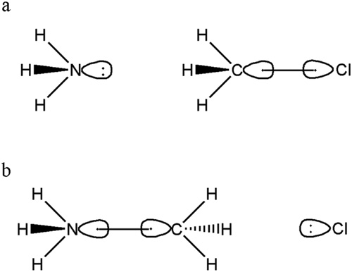
Fig. 2.3.1 Lewis structure for the reactant (a) and product (b).
2.3.4. Basis set and its subsets based on orbital symmetry
6–31G* is the basis set used in this example. The basis functions are simply separated into subsets according to the atoms. The basis functions on each atom will be treated as a subset and the VB orbitals will be built with these subsets.
2.3.5. Structures
There are 6 VB structures involved in the active space as shown in the figure. Structures S1-S3 describe the reactant, and S3-S5 describe the product. S6 describes the electron transfer between NH3 and Cl, and will appear in the TS region.
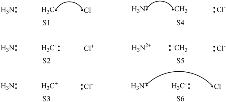
Fig. 2.3.2 6 VB structures for Menshutkin Reaction.
2.3.6. Input File
The input files of L-VBSCF for reactant and TS are given below:
Reactant:
NH3CH3cl reactant
$ctrl
vbscf
nmul=1 nstr=6 iscf=5 nao=3 nae=4
orbtyp=hao frgtyp=atom
int=libcint basis=6-31G*
guess=read
$end
$stru
1:16 17 17 18 19
1:16 17 17 18 18
1:16 17 17 19 19
1:16 18 18 17 19
1:16 19 19 17 18
1:16 18 18 19 19
$end
$orb
1*5 4 4 1*3 4*3 4*3 4 4 1
6
6
6
6
6
1 7 8 9
2 3 4 5
6
6
6
1 7 8 9
1 7 8 9
1 7 8 9
2 3 4 5
2 3 4 5
2 3 4 5
1 7 8 9
2 3 4 5
6
$end
$geo
 N      0.000000    0.000000    0.000000
 C      0.000000    0.000000   10.000000
 H     -1.029985    0.000000    9.647297
 H      0.514992    0.891993    9.647297
 H      0.514992   -0.891993    9.647297
 Cl     0.000000    0.000000   11.778400
 H      0.939678    0.000000   -0.389227
 H     -0.469839    0.813785   -0.389227
 H     -0.469839   -0.813785   -0.389227
$end
TS:
NH3CH3cl
$ctrl
vbscf
nmul=1 nstr=6 nao=3 nae=4 iscf=5 itmax=300
guess=read orbtyp=hao frgtyp=atom
int=libcint basis=6-31G*
$end
$stru
1:16 17 17 18 19
1:16 17 17 18 18
1:16 17 17 19 19
1:16 18 18 17 19
1:16 19 19 17 18
1:16 18 18 19 19
$end
$orb
1*5 4 4 1*3 4*3 4*3 4 4 1
6
6
6
6
6
1 7 8 9
2 3 4 5
6
6
6
1 7 8 9
1 7 8 9
1 7 8 9
2 3 4 5
2 3 4 5
2 3 4 5
1 7 8 9
2 3 4 5
6
$end
$geo
N    0.0000000000   0.0000000000  -2.4403680000
C    0.0000000000   0.0000000000  -0.6327610000
H    1.0651490000   0.0000000000  -0.4753840000
H   -0.5325745000  -0.9224460928  -0.4753840000
H   -0.5325745000   0.9224460928  -0.4753840000
CL   0.0000000000   0.0000000000   1.8067450000
H   -0.9550790000   0.0000000000  -2.8031240000
H    0.4775395000   0.8271226766  -2.8031240000
H    0.4775395000  -0.8271226766  -2.8031240000
$end
The input files are almost the same except the initial guess and geometry. The initial guess of reactant is given here. The initial guess of TS can be obtained from the computational results of reactant. For L-BOVB computations, the user may simply change ISCF=5 to ISCF=2 and append BOVB in $CTRL section. The initial guess of L-BOVB computations are from the computational results of correpsonding L-VBSCF computation.
2.3.7. Computational Results
2.3.7.1. The VB structures
Following table shows the VB structures involved in the calculation. The first 16 doubly occupied orbitals are inactive ones, orbital 17 corresponds to the lone pair on NH3, and orbitals 18 and 19 are singly occupied orbitals on CH3 and Cl respectively. The correspondence to the structures is also listed.
VB structure |
Structure |
|---|---|
1 ***** 1:16 17 17 18 19 |
S1 |
2 ***** 1:16 17 17 18 18 |
S2 |
3 ***** 1:16 17 17 19 19 |
S3 |
4 ***** 1:16 18 18 17 19 |
S6 |
5 ***** 1:16 19 19 17 18 |
S4 |
6 ***** 1:16 18 18 19 19 |
S5 |
2.3.7.2. Energies
Following table shows the total energies (in a.u.) and reaction barrier at the L-VBSCF and L-BOVB levels. Compared with the reference value 33.0 kcal mol -1 (138.1 kJ mol -1) by Webb and Gordon, L-VBSCF overestimates the reaction barrier due to the lack of dynamic correlation, and L-BOVB significantly improves the result. Compared with the energies obtained by L-VBSCF and L-BOVB, L-BOVB decreases the energy at the TS geometry much more than in the reactants. The results show that dynamic correlation plays an important role in reaction barrier calculations.
L-VBSCF |
L-BOVB |
|
|---|---|---|
\(E^{react}_{tot}\) |
-555.27775 |
-555.29156 |
\(E^{TS}_{tot}\) |
-555.21152 |
-555.24558 |
\(\Delta E^\neq\) |
41.6 |
28.8 |
2.3.7.3. VB wavefunction and weights
Table shows the weights of VB structures in the reactant and TS geometries. It is clear that the most important contribution comes from S1 in the reactant geometry and S3 in the TS geometry. In the TS, S4 represents the “covalent” structure of product and S3 represents the major “ionic” structure in both reactant and product. Thus, S3 represents the “bond breaking” of C-Cl and S4 shows the “bond forming” of N-C. Similar to the previous examples, L-BOVB provides larger weights for the secondary ionic structures as compared with L-VBSCF weights, which indicates that dynamic correlation plays a more important role for ionic structures than covalent ones, as already explained.
Reactant |
TS |
|||
|---|---|---|---|---|
L-VBSCF |
L-BOVB |
L-VBSCF |
L-BOVB |
|
S1 |
0.663 |
0.621 |
0.091 |
0.178 |
S2 |
0.105 |
0.120 |
-0.001 |
0.002 |
S3 |
0.232 |
0.259 |
0.532 |
0.487 |
S4 |
0.000 |
0.000 |
0.364 |
0.286 |
S5 |
0.000 |
0.000 |
-0.004 |
0.010 |
S6 |
0.000 |
0.000 |
0.017 |
0.037 |
2.4. Potential Energy Surface of LiF (Optional)
2.4.1. Introduction
LiF is a simple hetero diatomic molecule with a single bond between atoms Li and F. The dissociation of LiF is always in the interest of chemists. The so-called “Harpoon effect” makes electron transfer when the distance between Li and F even larger than the sum of their van der Waals radius, indicating an electron transfer due to the crossing of diabatic states. For details, please refer to the reference.
In this optional exercise, the user should compute a series of points along the dissociation of LiF, get the energies of total wave function and each VB structure, and plot the potential energy surface. This exercise should be done by the users themselves. Only essential clues will be given. The basis set in this exercise is cc-pVDZ, and the active space is the minimal space.
2.4.2. Computations near equilibrium
The distance RLi-F is set to 1.5 Angstrom.
2.4.2.1. Computation with all VB structures
Note
There is only a single bond in the molecule, so the minimal active space should be (2,2).
VB structures can be automatically generated as we have seen in the example of F2.
Use keywords
ORBTYP=HAOandFRGTYP=SAOwith proper definition of fragmenets in$FRAGto build the orbitals.The active orbitals should always be placed at the last in
$ORBsection.
2.4.2.2. Computation with all possible covalent structures
Note
The covalent VB structures can be either picked from all VB structure computation, or generated automatically.
Orbitals obtained in previous computation can be used as initial guess.
2.4.2.3. Computation for all possible Li+ F- ionic structures
Note
VB structures can be picked from all VB structure computation.
Initial guess can be obtained from the orbitals of previous computation.
2.4.2.4. Computation for all possible Li- F+ ionic structures
Note
VB structures can be picked from all VB structure computation.
Initial guess can be obtained from the orbitals of previous computation.
2.4.3. Computations for Other distances
Repeat the above computations at RLi-F = 1.1, 1.3, 1.7, 2.0, 2.6, 2.8, 3.0, 4.0, 7.0 Angstrom, get the energies and plot the potential energy surface. See at which distance the diabatic states cross. Following is the example of the potential energy surface.
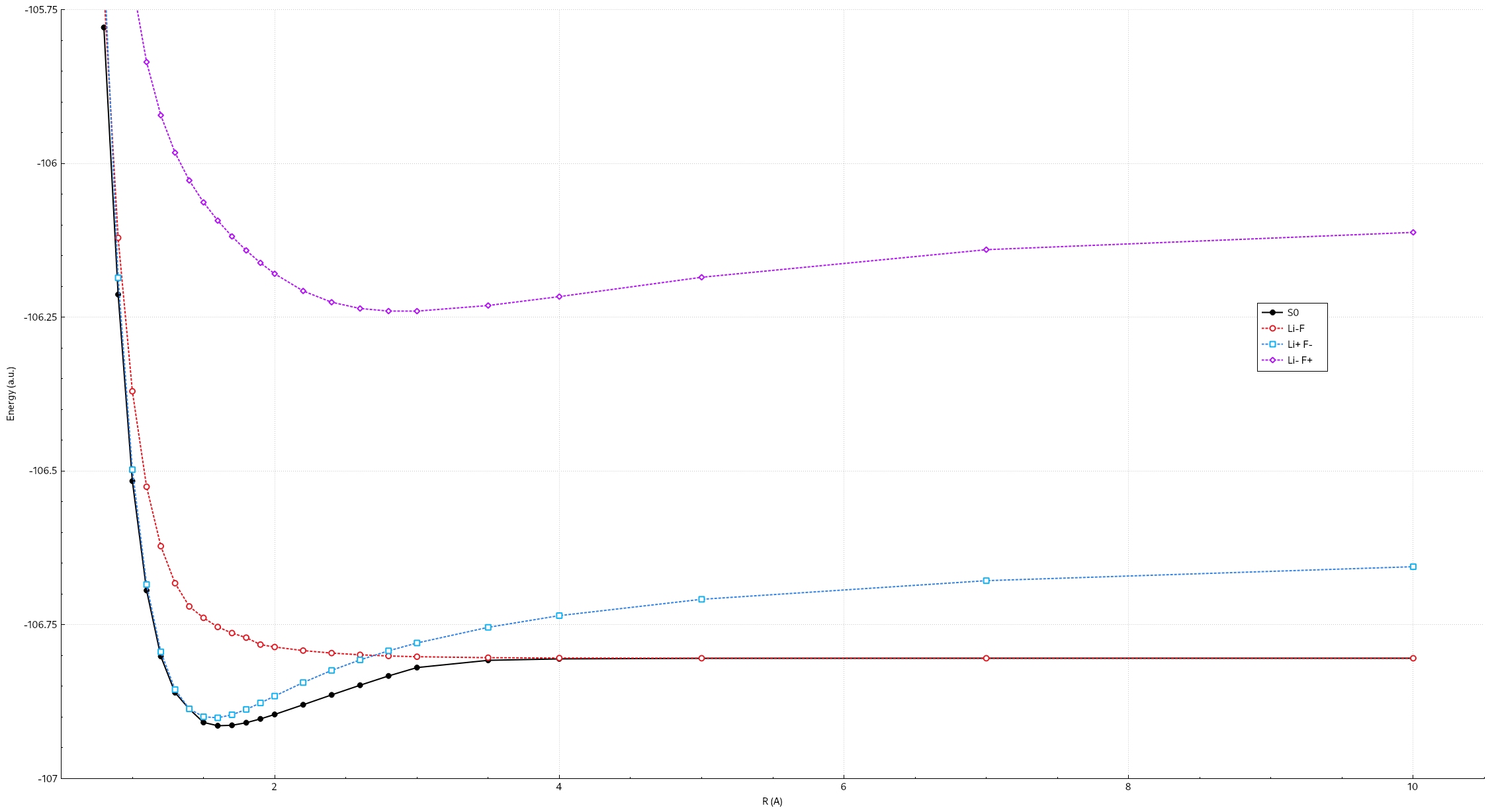
Fig. 2.4.1 Potential Energy Surface of LiF with cc-pVDZ
3. Citation
You need to cite the references of XMVB as following formats:
A) J. Chem. Phys. format: The ab initio Valence Bond calculations are performed with the XMVB program.
B) American Chemical Society format: The ab initio Valence Bond calculations are performed with the XMVB program.