Input
The extension name of XMVB input file is “xmi”. All the contents is organized in sections and case insensitive. The input file is structured in sections with following rules:
The first line of an xmi file is the job title or description of the job and should not be replaced or omitted.
A section start with a line includnig only the section name and ends with a line with only “$END”.
All contents after “#” is recognized as a comment and will not be parsed.
Commonly used sections are:
A typical example of XMVB input file is shown below. The user may download the input file with detailed explaination here.
H2 L-VBSCF
$CTRL
VBSCF
NSTR=3
NAO=2 NAE=2
ORBTYP=HAO FRGTYP=SAO
INT=LIBCINT
BASIS=CC-PVTZ
$END
$STR
1 2
1 1
2 2
$END
$FRAG
1 1
SPZDXXDYYDZZ 1
SPZDXXDYYDZZ 2
$END
$ORB
1 1
1
2
$END
$GEO
H 0.0 0.0 0.0
H 0.0 0.0 0.74
$END
$GUS
15 15
# ORBITAL 1 NAO = 15
-0.3532245024 1 -0.5363311264 2 -0.2343104477 3 -0.0000000000 4
 0.0000000000 5 -0.0199961314 6 -0.0000000000 7  0.0000000000 8
-0.0192894825 9 -0.0003896018 10 0.0000000000 11 -0.0000000000 12
-0.0003896018 13 0.0000000000 14 -0.0020820012 15
# ORBITAL 2 NAO = 15
 0.3532245024 16 0.5363311264 17 0.2343104477 18 0.0000000000 19
-0.0000000000 20 -0.0199961314 21 0.0000000000 22 -0.0000000000 23
-0.0192894825 24 0.0003896018 25 -0.0000000000 26 -0.0000000000 27
0.0003896018 28 0.0000000000 29 0.0020820013 30
$END
Global control ($CTRL)
The $CTRL section contains the information of how a job is performed. The input format is name=value or name=option, except for the keywords which need no values or options. <enter> and <space> are used to separate keywords. If a keyword accepts several options in a time, the options are separated with “,”.
Keywords for Global Control
UNIT=option
The unit for geometry in $GEO. Available options are:
* ANGS: Geometry is given in Angstroms. This is the default option.
* BOHR: Geometry is given in Bohr.
ITMAX=n
n is the maximum number of iterations. Default value is 200.
NMUL=n
n is the spin multiplicity (2S + 1) of system. Default value is 1, which means singlet state.
NAO=m
m is the number of active VB orbitals whose occupation number varies in the structures. NAO is required if keywords STR or ISCF=5 (see below) is specified.
NAE=n
n is the number of active VB electrons which occupy the active orbitals. NAE is required if keywords STR or ISCF=5 (see below) is specified.
NSTR=n
n is the number of VB structures (or determinants). This keyword can be omitted if STR (see below) is assigned.
STR=options
This keyword generates VB structures automatically and hence NSTR and the $STR section are not needed. This keyword requires NAO and NAE to declare the active space. Users may use one or several of the following options:
COV: Covalent structures will be generated.
ION[(n-m)]: Ionic structures will be generated. A simple ION will generate all ionic structures; ION(n,m) will generate only the \(n^\textrm{th}\) and \(m^\textrm{th}\) order ionic structures and ION(n-m) will generate ionic structures from the \(n^\textrm{th}\) to the \(m^\textrm{th}\) order.
FULL: All VB structures will be generated.
FIXC
Request to fix structure coefficients for VB structures. In VB theory, the coefficients are obtained by solving the secular equation
For some special purposes, one may want to fix the coefficients. In such situation, the coefficients are inputted following the corresponding VB structures and the energy will be obtained directly by
For example, the following input will constrain the coefficients of the three VB structures to be 1.0:0.5:0.5
$STR
1 2 1.0
1 1 0.5
2 2 0.5
$END
The corresponding wave function will in the expression
where N is the normalization coefficient.
GROUP=EXP
Divide VB structures into groups according to the expression EXP. An expression with n structures divided into m groups can be expressed as:
Here \(S_{i1} \ldots S_{nm}\) are the structure numbers, a comma “,” is used to separate the structures numbers in the same group, and two commas “,,” is used to separate different groups. Coefficients of structures should be given in Global control ($CTRL), similar to FIXC. The ratio of VB structures within the same group will be fixed, as introduced in FIXC. The coefficients of VB structures in different groups will not be fixed and shall be optimized by solving secular equation. Following is an example:
$CTRL
NSTR=3
GROUP=1„2,3
$END
$STR
1 2 1.0 # S1
1 1 0.5 # S2
2 2 0.5 # S3
$END
The above example devide 3 VB structures into 2 groups:
Group 1. \(G_1 = S_1\)
Group 2. \(G_2 = 0.5(S_2 + S_3)\)
Hence a 3 structure problem becomes a 2 “structure” problem:
where \(C_1\) and \(C_2\) are coefficients of \(G_1\) and \(G_2\) obtained by solving secular equation. The finalwave function can be expressed as
NSTATE=n
Energy, coefficients and weights of structures for the \(n^\textrm{th}\) excited state, rather than for the ground state, will be calculated and printed out. The values of n can be:
0: The ground state.(Default)
n: The \(n^\textrm{th}\) excited state.
Note
VB orbitals are optimized by minimizing the energy of required state. When the \(n^\textrm{th}\) excited state is requested, the \((n+1)^\textrm{th}\) root will be chosen as the \(n^\textrm{th}\) excited state when solving the secular equation. Thus, n must be smaller than the number of structures.
For VBCI calculaitons, NSTATE can be only 0 or 1.
SORT
Sort the VB structures in descending order according to coefficients.
CTOL=tol
Set the Coefficient TOLerance when printing coefficients and weights of VB structures.
Only the coefficients and weights of VB structures whose absolute values of coefficients are not smaller than tolerance tol will be printed. The default tolerance is 0, which means all structures will be printed.
Note
The tolerance tol is a real parameter. For instance,
CTOL=0.01
means that only structures whose absolute values of coefficients larger than or equal to 0.01 will be printed. For VBCI this keyword is not functioning
CICUT=n
Set cut threshold to \(10^{-n}\) for CI configurations. The contribution of a CI configuration is estimated by perturbation theory. If the contribution is less than the threshold, the configuration will be discarded. This will reduce the computational effort for CI calculations. Recommended values are 5 or 6. Default value is 0 (no cut).
NCOR=m
In VBCI or VBPT2 calculations, the first m orbitals (2m electrons) will be frozen in the VBCI or VBPT2 calculation. In BOVB caluclations, the first m orbitals will be kept as VBSCF orbitals. The default value is 0, which means all orbitals will be counted in VBCI, VBPT2 or BOVB.
GUESS=option
This keyword describes the way to generate or read the initial guess for a VB computation.
Valid options can be:
AUTO: The program automatically provides guess orbitals by diagonalizing a fragmant-localized Fock matrix. This is the default option.
UNIT: The first basis function of an orbital in $ORB is set to be the guess for the orbital.
MO: Initial guess will be obtained from MOs.
READ: Guess orbitals are read from external file, which should be provided by user.
Note
The Initial guess description ($GUS) section is required when
GUESS=MOorGUESS=READis specified. Note that the format of the Initial guess description ($GUS) section differs depending on whetherGUESS=READorGUESS=MOis used. Detailed explanations for both formats are provided in the Initial guess description ($GUS) section documentation.To enhance user convenience and ensure reliable calculations, the software automatically detects whether the format in the Initial guess description ($GUS) section corresponds to
GUESS=READorGUESS=MO. Therefore, if the Initial guess description ($GUS) section is included, theGUESSkeyword can be omitted when using either of these two options.
WFNTYP=option
Options for the way to expand the many-electron wave functions of system.
STR: VB structures are used. (Default)
DET: VB determinants are used for state functions, instead of VB structures.
ORBTYP=option
Specify the type of VB orbitals. Valid options are:
HAO: Hybrid Atomic Orbitals are used.
OEO: Overlap Enhanced Orbitals are used.
GEN: VB orbitals are defined by users. The orbitals will be described in terms of basis functions explicitly in Orbital description ($ORB) section. (Default)
Note
Fragments definition ($FRAG) is needed if
ORBTYP=HAOis specified. The Fragments definition ($FRAG) section will specify the fragments based on atoms or basis functions and orbitals will be assigned in Orbital description ($ORB) section based on the fragment definitions in Fragments definition ($FRAG).ORBTYP=OEOdoes not need Fragments definition ($FRAG) and Orbital description ($ORB) sections since the OEOs are delocalized in the whole system.ORBTYP=GENdoes not need Fragments definition ($FRAG) section.
FRGTYP=option
Specify the type of fragments when ORBTYP=HAO.
ATOM: The fragments of system will be defined with atoms. This is the default.
SAO: The fragments of system will be defined with symmetrized atomic orbitals.
Note
Fragments definition ($FRAG) is required for FRGTYP=SAO. For FRGTYP=ATOM, each atom is considered as a fragment if no FRAG section appears in the input file.
Tip
In addition to assigning all orbitals in the Orbital description ($ORB) section, the software supports a simplified input format that requires only the active orbitals to be assigned while using the default options for ORBTYP and FRGTYP. For more details, refer to the Active orbital description ($ACTORB) section.
FRZORB=EXP
Specify the indices of orbitals to be frozen. Frozen orbitals will not be optimized in the calculation. Following is an example for frozing orbital 1, 3, 5, 6 and 7
$CTRL
FRZORB=1,3,5-7
$END
Note
This keyword is only available for VBSCF calculation currently.
Keywords for Computational Methods and Algorithms
HF/RHF/UHF/ROHF
A Hartree-Fock calculation will be proceeded. RHF/UHF/ROHF represent the restricted, unrestricted and restricted open-shell Hartree-Fock calculations respectively. When only “HF” is assigned, RHF will be proceeded when system is singlet and UHF for other cases.
Density Functional Theory
A DFT calculation will be proceeded. Currently supported keywords and corresponding functionals are listed below:
- GGA Functionals
BLYP Becke88 + Lee-Yang-Parr XC functional
PBE Perdew-Burke-Ernzerhof XC functional
PW91 Perdew-Wang 1991 XC functional
- Hybrid Functionals
BHHLYP 0.5 B88 + 0.5 HFX + LYP hybrid functional
B3LYP Becke’s 3 parameter hybrid functional
B3LYP-D3 B3LYP with D3 dispersion correction
B3LYP-D3BJ B3LYP-D3 with damping
PBE0 A hybrid with 25% exact exchange and 75% DFT exchange made from PBE
The users may use “R”, “U”, and “RO” ahead of the name of functional to specify restricted, unrestricted or restricted open-shell calculations, the same as HF method. For example, “RB3LYP” will run the restricted B3LYP calculation. If only the name of functional is specified, restricted calculation will be run for singlet and unrestricted for others.
VBSCF
A VB Self-Consistent Field computation is requested. This is the default method for the XMVB program.
BOVB
Ask for a Breathing Orbital VB (BOVB) calculation.
Note
BOVB method cannot be used with VBCI.
BOVB method is usually more difficult to converge than VBSCF. Thus, it is recommended to run a BOVB job with a good initial guess. It is recommended to run a VBSCF calculation first, followed by the BOVB calculation with optimized VBSCF orbitals as the initial guess.
VBCIS:
Ask for a VBCIS calculation.
VBCISD
Ask for a VBCISD calculation.
VBPT2
A VBPT2 computation will be performed.
HC-DFVB=func
Ask for an HC-DFVB calculation. func is the DFT functional used for DFVB computation. Currently BLYP, B3LYP, B3LYP5, BHHLYP, PW91, PBE, and PBE0 functionals are available.
LAM-DFVB=func
Ask for an λ-DFVB(U) calculation. func is the DFT functional used for DFVB computation. Currently only BLYP functional is available.
MS-DFVB=func
Ask for an λ-DFVB(MS) calculation. func is the DFT functional used for DFVB computation. Currently only BLYP functional is available. Additionally, MS-DFVB has to be used with keyword WSTATE.
Note
The parameters used in the λ-DFVB(U) and λ-DFVB(MS) methods are specifically fitted for the VBSCF wave function of all structures with OEOs. Therefore, it is recommended to use STR=FULL and ORBTYP=OEO together with LAM-DFVB or MS-DFVB. While other combinations of STR and ORBTYP may also work with LAM-DFVB or MS-DFVB, these are not recommended, as no parameters are available for other wavefunction types.
TBVBSCF
Activate tensor-based VBSCF. Currently TBVBSCF is valid only when:
ISCF=5,NAO=mandNAE=nare selected.Structures are generated automatically with STR=options.
Number of active electrons should be at least 4, in which 2 for both \(\alpha\) and \(\beta\) parts.
ISCF=n
ISCF specifies orbital optimization algorithm. The value n currently can be:
2: Analytical gradients in terms of basis functions with the L-BFGS algorithm. This algorithm involves only the first-order density matrix and is the default for BOVB.
5: Analytical gradients in terms of VB orbitals with the L-BFGS algorithm. This is the most efficient algorithm so far. Keywords
NAOandNAEare needed. This is the default for VBSCF.6: VBSCF with full hessian matrix.
NAOandNAEare needed for this option. This algorithm is potentially faster and more robust than ISCF=5, but it is still under development and thus is not recommended in the current version of the program.
WSTATE=EXP
Activate the state-average VBSCF/BOVB calculation. WSTATE may provide an array containing non-zero weights of the specific states. Following is the example for
$CTRL
NSTR=10 WSTATE(3)=0.5,0.0,0.3,0.0,0.0,0.2
$END
Note
WSTATE currently cannot be used with TBVBSCF and ISCF=6.
Keywords for Integrals
INT=option
Read integrals from file or calculate them directly. The valid options can be:
LIBCINT: Integrals are calculated directly by an external library LIBCINT. Section Geometry description ($GEO) is essential. This is the default option.
RI: 2-e integrals are evaluated with resolution identity (RI).
COSX: 2-e integrals are evaluated with grid-based COSX.
READ: Read integrals from existing files “x1e.int”, “x2e.int” and “INFO”.
Note
Note that he absolute energies vary depending on the integral type used. Therefore, ensure that the relative energy is calculated using the same integral type for consistency.
BASIS=basis_set
Assigning the basis set when INT=CALC is requested. Basis sets are expressed the same way as Gaussian, i.e. 6-31G*, aug-cc-pVTZ etc. The supported basis sets can be found in Basis sets in XMVB.
NCHARGE=n
Charge of the system in current XMVB calculation. Default is 0, which means the neutural system. Positive numbers denote a cation system and negative numbers mean the system is anion. This keyword will also specify the number of electrons in current calculation, NEL is not needed anymore in such case.
Keywords for Wave Function Analysis
BOYS
Boys localization is requested for the final VB orbitals.
Note
It is strongly recommended to use this keyword for VBSCF. This makes VB orbitals easier to be interpreted and more physically meaningful.
Boys localization is available only for VBSCF method.
Boys localization can be only used in cases in which orbitals are separated into blocks, and there is no common basis function between blocks.
OUTPUT=AIM
WFN file for AIM2000 program will be printed. A $AIM with WFN filename is relevant for this keyword. This is not available if INT=READ is assigned.
MOLDEN
MOLDEN file will be punched with name input.molden in which input is the input file name. This file can be used to visualize the geometry and VB orbitals. Cannot be used with INT=READ.
VBCAD[=option]
Diabatization procedure VBCAD will be proceeded after VBSCF or BOVB computation. Currently only 2-state diabatization is supported. VBCAD separates two diabatic states by maximizing the weights different of VB structures.
Users may use one of the following options:
C2: The square of coefficients of VB structures will be used instead of weights of VB structures. This is the default option.
CC: The Coulson-Chirgwin weights will be used.
RE: The Renormalize weights will be used.
LOWDIN: The Löwdin weights will be used.
INV: The Inverse weights will be used.
n: Input number instead of name of weights.
1is a synonym ofC2,2is a synonym ofCC,3is a synonym ofRE,4is a synonym ofLOWDIN,5is a synonym ofINV.
CADGRID=n
The step size for searching the givens rotation angle that maximizing the weights different of VB structures in degree. The default is 0.5 degree.
Note
The keyword CADGRID needs to be used together with VBCAD. However, the default options has been extensively used and they all result in well-separated diabatic states. So it is recommended to simply use the VBCAD keyword alone.
The CADGRID keyword is intended to be used with VBCAD. However, due to the extensive use of default settings, which result in well-separated diabatic states, it is recommended to use the VBCAD keyword on its own.
Keywords for Geometry Optimization
Following are the keywords for geometry optimization. Keywords in this section is only available for VB computations with INT=LIBCINT. Currently only global minima optimization with no constraint is supported.
OPT
A geometry optimization will be performed in Cartesian coordinates. Currently geometry optimization is only available for the VBSCF method (ISCF=5 or ISCF=6).
HESS=option
Options for evaluating initial Hessian used in geometry optimization. Currently following options are available:
GUESS: Initial Hessian is evaluated by a “guess” procedure based on some empirical parameters. This is the default option.
SEMINU: A semi-numerical procedure is used to evaluate initial Hessian. In this procedure, the gradient is evaluated analytically and Hessian is numerical based on analytical gradients.
FULLNU: A fully numerical procedure is used to evaluate initial Hessian. Both Hessian and gradient will be evaluated in purely numerical way.
MAXCYCLES=n
The maximum cycles for geometry optimization. The default is the maximum between 20 and 6*N, where N is the number of atoms.
GRADIENT
Geometrical gradient will be evaluated for current geometry but not for optimization.
Geometry optimization using Gaussian’s optimizer
To enable geometry optimization using Gaussian’s optimizer, use the keyword OPT=GAUSSIAN(NOMICRO[, ...]). The option NOMICRO activates a faster optimization approach and is recommended. The options within the parentheses correspond to those of the Opt keyword in Gaussian. When using Gaussian’s optimizer for geometry optimization, the Geometry description ($GEO) section must be provided in Gaussian format. The format for specifying fixed atoms or variables is the same as in Gaussian. Below is an example for optimizing the HCN molecule using internal coordinates, where the bond length B2 and bond angle A1 are held fixed, while bond length B1 is optimized.
$CTRL
OPT=GAUSSIAN(nomicro,z-matrix)
$END

$GEO
H
C   1  B1
N   2  B2  1  A1

B1=1.07

B2=1.1466
A1=179.999
$END
Note
This keyword is available on the XACS cloud only.
VB Structure description ($STR)
The $STR section describes the information of VB structures or VB determinants if DET of $CTRL section is specified. For VB structures, paired electrons, which may be lone pairs or covalent bonds, should be written first followed by unpaired electrons. The number of unpaired electrons depends on the spin multiplicity. For example: For a structure with three lone pairs (orbitals 1, 2, and 3), one covalent bond (orbitals 4 and 5), and one unpaired electron (orbital 6), the structure is expressed as,
1 1 2 2 3 3 4 5 6
For determinants, all alpha orbitals are listed first, followed by beta orbitals. For example: A determinant of alpha orbtials 1, 2, 3, 4, and 6 and beta orbtials 1, 2, 3, and 5 is expressed as
1 2 3 4 6 1 2 3 5
Note that it is strongly recommended to write the most important structure as the first one.
This can avoid potential problems in VBCI.
If BOVB is specified in $CTRL section, the program will try to convert the VB orbitals into breathing orbitals. It uses automatically different orbitals for different structures. For example: If the initial VB structures are:
1 1 2 3
1 1 2 4
1 1 3 5
The program will convert them to:
1 1 2 3
6 6 7 4
8 8 9 5
Note that the VB structures should be independent. VB structures are recommended to be written in the following orders:
Inactive Active
where “Inactive” stands for the inactive orbitals which keep doubly occupied in all structures; “active” stands for the active orbitals whose occupation varies in the structures. The singly occupied orbitals in high-spin systems should always be put in the tail of the structures.
Following are the examples of typical bonding patterns and their corresponding VB Structure description ($STR) and Global control ($CTRL) sections, in which only active orbitals are labeled:
System of 2-electrons on 2-centers
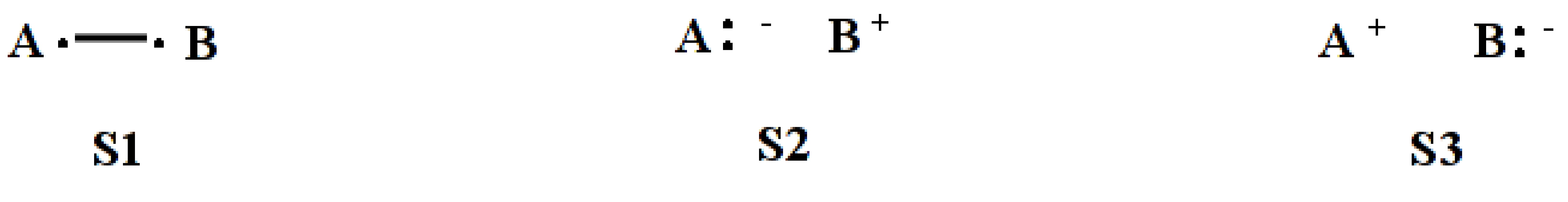
$CTRL
nstr=3 nmul=1
$END
$STR
1 2 ; S1
1 1 ; S2
2 2 ; S3
$END
System of 3-electrons on 2-centers
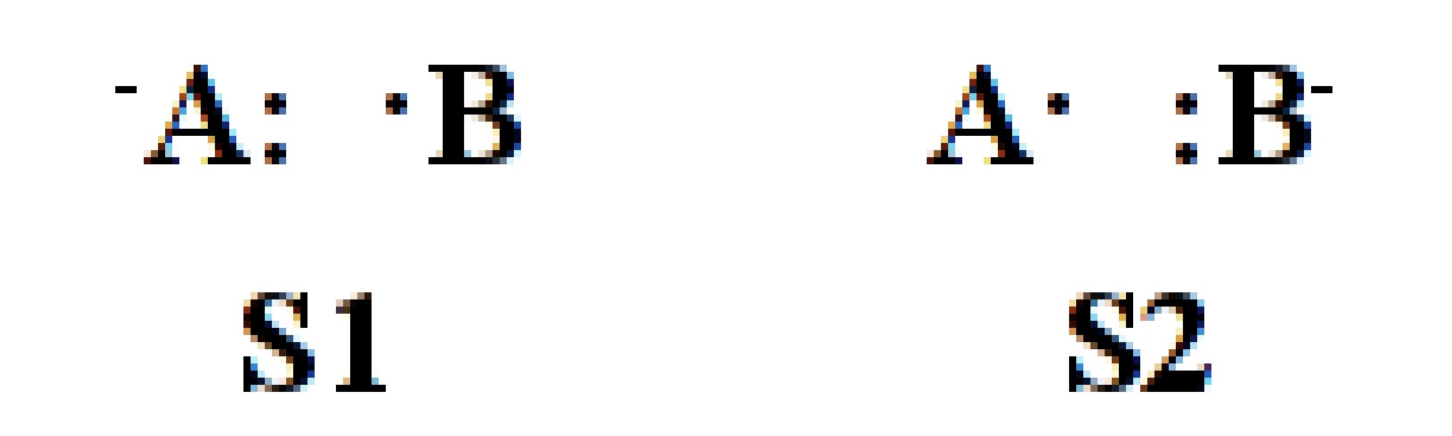
$CTRL
nstr=2 nmul=2
$END
$STR
1 1 2 ; S1
2 2 1 ; S2
$END
System of 3-electrons on 3-centers
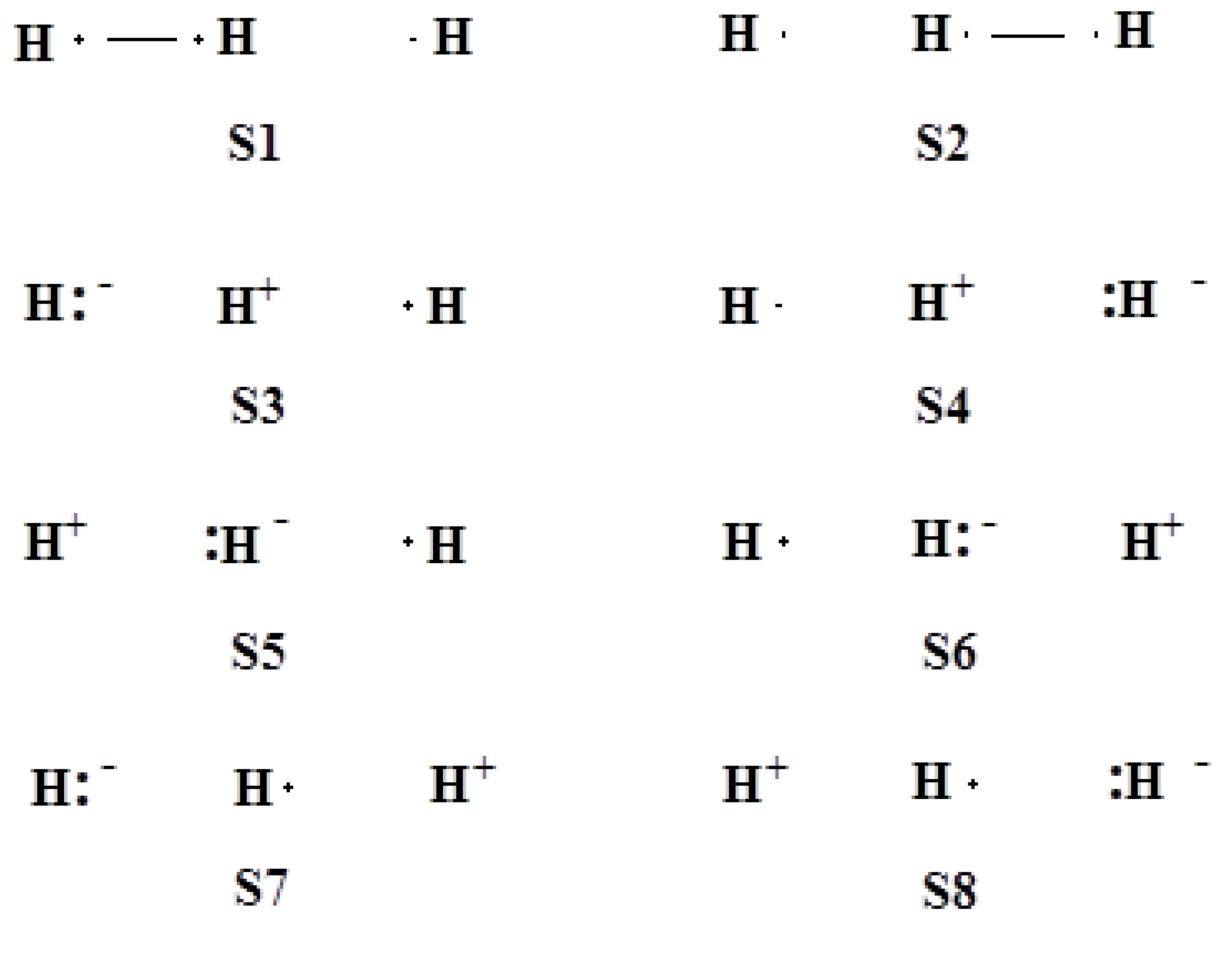
$CTRL
nstr=8 nmul=2
$END
$STR
1 2 3 ; S1
2 3 1 ; S2
1 1 3 ; S3
3 3 1 ; S4
2 2 3 ; S5
2 2 1 ; S6
1 1 2 ; S7
3 3 2 ; S8
$END
System of 4-electrons and 3-centers
6 VB structures (3 VB orbitals with 4 electrons, singlet)
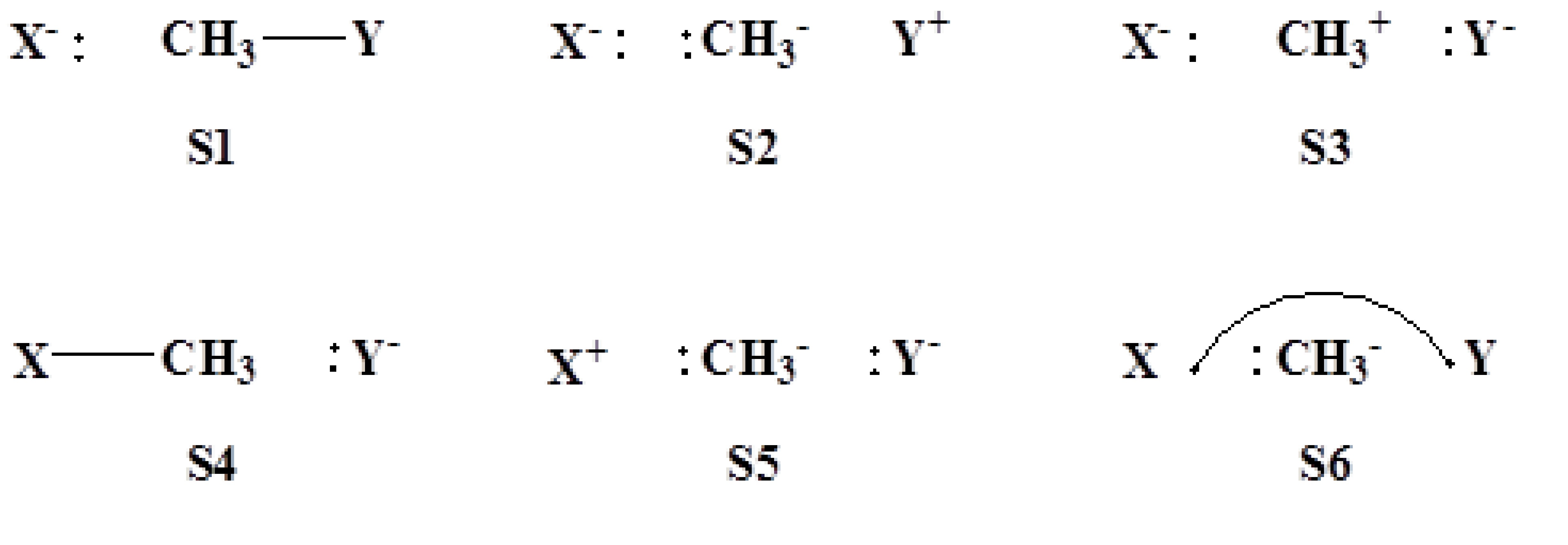
$CTRL
nstr=6 nmul=1
$END
$STR
1 1 2 3 ; S1
1 1 2 2 ; S2
1 1 3 3 ; S3
1 2 3 3 ; S4
2 2 3 3 ; S5
2 2 1 3 ; S6
$END
Note
- In XMVB 4.0, VB structures are represented in a new style in the output file for better readability. For VB structures, the inactive part is shown in the format of “1:X”, where “X” is the number of inactive orbitals. In the active part, ionic pairs are shown in the format “X X” where “X” is the doubly occupied orbital, and a covalent bond is shown as “X-Y”, where “X” and “Y” are orbitals between which covalent bonding is made. High spin electrons (if there are) are always shown at last.
For example, the covalent structure “2 2 1 3” will be shown as 2 2 1-3 in the output file.
Fragments definition ($FRAG)
Generally, the $FRAG section is required if ORBTYP=HAO. In this section, fragments in which VB orbitals are localized will be defined and the orbitals will be generated with the basis functions specified in the fragments.
The syntax of $FRAG is:
$FRAG
nf(1), nf(2), . . . nf(N)
[basis function description(1)] lf(1,1), lf(2,1), . . . lf(nf(1),1)
[basis function description(2)] lf(1,2), lf(2,2), . . . lf(nf(2),2)
. . .
[basis function description(N)] lff(1,N), lf(2,N), . . . lf(nf(N),N)
$END
Here the system is separated into N fragments. nf(i) means the number of atoms or basis functions in the \(i^\textrm{th}\) fragment, and lf(j,i) is the atom or basis function j in the \(i^\textrm{th}\) fragment. Basis function description is needed only when FRGTYP=SAO is chosen. Following is an example of H2 molecule with FRGTYP=ATOM:
$CTRL
NSTR=3 ORBTYP=HAO
FRGTYP=ATOM
$END
$STR
1 2
1 1
2 2
$END
$FRAG
1 1
1
2
$END
$ORB
1 1
1
2
$END
The above $FRAG specifies two fragments, where one atom is in each fragment. Fragment 1 includes the first H atom and fragment 2 includes the second H atom. With this definition, users only need to specify fragment in which an orbital is located in Orbital description ($ORB) section. With FRGTYP=SAO, the fragments are specified by the type of basis functions. Following is an example of HF molecule with 6-31G basis set:
$CTRL
NSTR=3 VBFTYP=DET DEN
ISCF=5 NAO=2 NAE=2
ORBTYP=HAO FRGTYP=SAO
$END
$STR
1:4 5 6
1:4 5 5
1:4 6 6
$END
$FRAG
1 1 1 1
S 1
SPZ 2
PX 2
PY 2
$END
$ORB
1 1 1 1 1 1
2
2
3
4
2
1
$END
For the second fragment, “1” in the first line of $FRAG means that the block contains basis functions located on one atom; “SPZ 2” means that the fragment includes the \(s\) and \(p_z\) basis functions in the second atom. The basis functions are described by groups of \(s\), \(p\), \(d\), \(f\), etc. For example, a fragment including \(s\), \(p_z\), \(d_{xx}\), \(d_{yy}\), \(d_{zz}\), \(f_{zzz}\), \(f_{xxz}\) and \(f_{yyz}\) basis functions in atoms 1 and 2 should be described as
$FRAG
2
spzdxxyyzzfzzzxxzyyz 1 2
$END
or
$FRAG
2
spzdxxdyydzzfzzzfxxzfyyz 1 2
$END
Here “s” means basis function \(s\), “pz” means basis function \(p_z\), “dxxyyzz” means \(d_{xx}\), \(d_{yy}\) and \(d_{zz}\), and “fzzzxxzyyz” means \(f_{zzz}\), \(f_{xxz}\) and \(f_{yyz}\). The ordering of basis functions are not compulsively defined, but the basis functions with the same type of \(s\), \(p\), \(d\) and \(f\) should be written together. For example, the above description can be written equivalently as
$FRAG
2
spzfzzzfxxzfyyzdxxdyydzz 1 2
$END
or
$FRAG
2
spzfxxzfyyzfzzzdxxdyydzz 1 2
$END
as users like.
Orbital description ($ORB)
This section is to specify how each orbital is expanded in terms of the chosen basis functions or fragments.
Required When ORBTYP=HAO or ORBTYP=GEN.
The first line describes the number of basis functions (or fragments) that are used for VB orbitals. For instance, max(i) means that the \(i^\textrm{th}\) orbital is expanded as max(i) functions (fragments), which are specified in the following lines. If the value of max(i) is 1, it means that the corresponding orbital will not optimized. From the second line, the indices of basis functions are listed, where one orbital begins with one new line. Following is example:
4 4 2
3 4 5 6 ; orbital 1 is expanded with 4 basis functions (fragments)
4 3 5 6 ; orbital 2 is expanded with 4 basis functions (fragments)
1 2 ; orbital 3 is expanded with 2 basis functions (fragments)
Note
It is suggested to write the most important basis function as the first one, as the program takes the first function as the “parent” function for the orbital if
GUESS=UNIT. This can avoid potential problems in convergence.If
ORBTYP=OEOis chosen, the$ORBis not needed. All the orbitals will be delocalized in the whole system, which means orbitals will use all basis functions.If the users want to freeze (not optimize) some orbitals in the calculation, simply assigning the number of basis functions (fragments) of the corresponding orbital to “0”. For example, “0*5 2 2” means that there are totally 7 VB orbitals and the first 5 will be frozen during SCF iterations. In this case, an initial guess should be provided either by
GUESS=READorGUESS=MO.
Active orbital description ($ACTORB)
The VB orbitals can be defined using the $ACTORB section as an alternative to the $ORB section.
In the $ACTORB section, only the active orbitals need to be specified, while inactive orbitals are automatically assigned as OEO by default.
Additionally, ORBTYP=HAO and FRGTYP=ATOM are automatically enabled in this case.
The $ORB section consists of m lines, where m represents the number of active orbitals.
Each line describes an active orbital, with the \(i^\textrm{th}\) line corresponding to the \(i^\textrm{th}\) active orbital.
For each line, users must specify the atom indices associated with the current orbital distribution.
An example of $ACTORB for F2 is shown here:
$ACTORB
1 ; 2pz orbital of F1
2 ; 2pz orbital of F2
$END
The settings above is the same as:
$CTRL
ORBTYP=HAO FRGTYP=ATOM
$END
$ORB
2*8 1*2
1 2 ; inactive orbital
1 2 ; inactive orbital
1 2 ; inactive orbital
1 2 ; inactive orbital
1 2 ; inactive orbital
1 2 ; inactive orbital
1 2 ; inactive orbital
1 2 ; inactive orbital
1   ; 2pz orbital of F1
2   ; 2pz orbital of F2
$END
Using $ACTORB can significantly simplify the input file, particularly for large molecules. For example, for the test calculation in λ-DFVB(MS) Calculation of the Spiro cation, the use of $ACTORB can simplify the $ORB section into:
$ACTORB
2  3  4  11 29 16 24 27
7  8  9  10 28 19 25 26
2  3  4  11 29 16 24 27
7  8  9  10 28 19 25 26
$end
Note
ORBTYP=HAOandFRGTYP=ATOMare automatically enabled when the $ACTORB` section is used. Therefore, Therefore, users can omit these two keywords when utilizing$ACTORB.The
$ACTORBsection and theORBsection are mutually exclusive.
AIM Section($AIM)
This section is relevant if OUTPUT=AIM is specified. The content of this section is an optional file name specified by users. This file name will be used as the WFN file name. By default, the content of WFN file will be stored in ".wfn" file with the same name as input.
Initial guess description ($GUS)
Required when GUESS=MO or GUESS=READ.
When GUESS=MO is required in Global control ($CTRL) section, $GUS describes how VB orbital guess comes from MOs. An example of $GUS from H2 calculation is shown below:
$GUS
1 1
2 1
$END
The example shows that both VB orbitals 1 and 2 will get the initial guess from MO 1. All orbitals should be specified in this section.
If GUESS=READ is required, orbitals from previous computation will be read from $GUS section. Thus, this section now contains the orbitals provided as the initial guess. The content is the same as the ORB file of the previous computation. See File with optimized VB orbitals (.orb) for details of the content.
Note
To enhance user convenience and ensure reliable calculations, the software automatically detects the content in $GUS. Refer to GUESS=option for details.
Therefore, if the $GUS section is included, the GUESS keyword can be omitted when using either GUESS=MO or GUESS=READ.
Geometry description ($GEO)
Required when INT=CALC or INT=LIBCINT.
section contains the geometry of the system in cartesian coordinates, and the unit is Angstrom. Both Gaussian and GAMESS-US format are supported. Here both examples of the same geometry are given:
Gaussian Format:
$GEO
F 0.0 0.0 -0.7
F 0.0 0.0 0.7
$END
GAMESS-US Format:
$GEO
F 9.0 0.0 0.0 -0.7
F 9.0 0.0 0.0 0.7
$END
The users may choose their favorite.