AIQM2

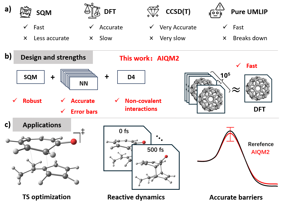
AIQM2 is the second generation of our AI-enhanced quantum mechanics methods (AIQM) series. Its high speed, competitive accuracy, and robustness enable organic reaction simulations beyond what is possible with the popular DFT methods. It can be used for transition state (TS) structure search and reactive dynamics, often with chemical accuracy. Except for energies, AIQM2 can also provide other molecular properties, e.g., dipole moment for generating infrared (IR) spectra.

More details can be found in our recent publication on Chemical Science:

Yuxinxin Chen, Pavlo O. Dral*. AIQM2: Organic Reaction Simulations Beyond DFT. Chem. Sci. 2025, accepted manuscript. DOI: 10.1039/D5SC02802G. Preprint on ChemRxiv: https://doi.org/10.26434/chemrxiv-2024-j8pxp (2024-10-08).

AIQM2 is already available in our open-source MLatom software. It is also one of the most frequently used methods on the Aitomistic Hub for online simulations via a web browser, including the AI assistant Aitomia. Although AIQM2 is limited to the CHNO elements, AIQM2@UAIQM is available for all but the 7th row elements. AIQM2 is available via PyPI and on GitHub, AIQM2@UAIQM as described in the UAIQM tutorial.

Topics to be covered in this tutorial include:

Start with Aitomistic Hub
Reactive molecular dynamics with AIQM2
IR spectra
Integrate implicit solvent in AIQM2
Solve convergence problem

Prerequisites

If you want to try AIQM2 locally, the following packages are required:

MLatom (https://github.com/dralgroup/mlatom, it’s recommmended to use the latest version of MLatom where we improved many functionalities of using AIQM2. The MLatom version should be greater than 3.12.0)
DFT-D4 (https://github.com/dftd4/dftd4, please use the pypi version and find the executable dftd4 under /bin folder of the environmnet)

After the installation of DFT-D4, you need to set the environment variable dftd4bin=[your DFT-D4 binary]

As an alternative, you can directly try AIQM2 on our online platform Aitomistic Hub without the need for environment installation. We will show how to run AIQM2 on Aitomistic Hub in the following tutorial. The required scripts are the same if you want to run locally.

Basics of Aitomistic Hub

First of all, there are four main regions in your workspace.

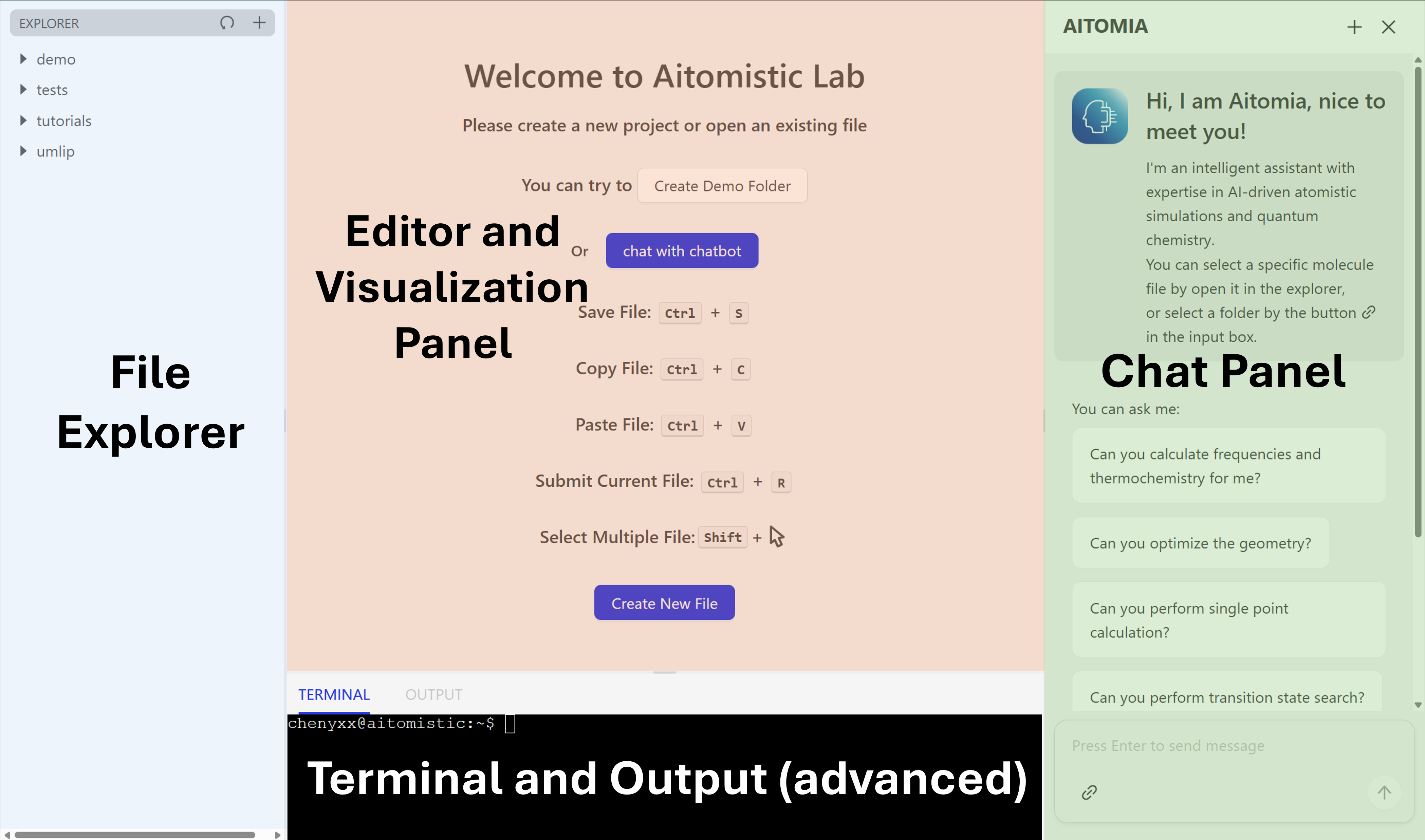
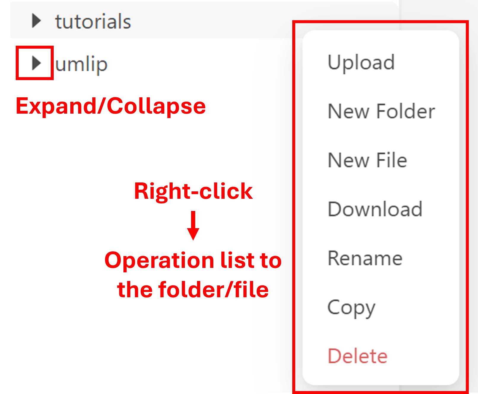
The core regions of the workspace on Aitomistic Hub

In the file explorer, you can copy, move and create files and folders. By right click on the file or folder, you can choose the options you want. The triangle symbol on the right side of the folder can be used for expansion and collapse.

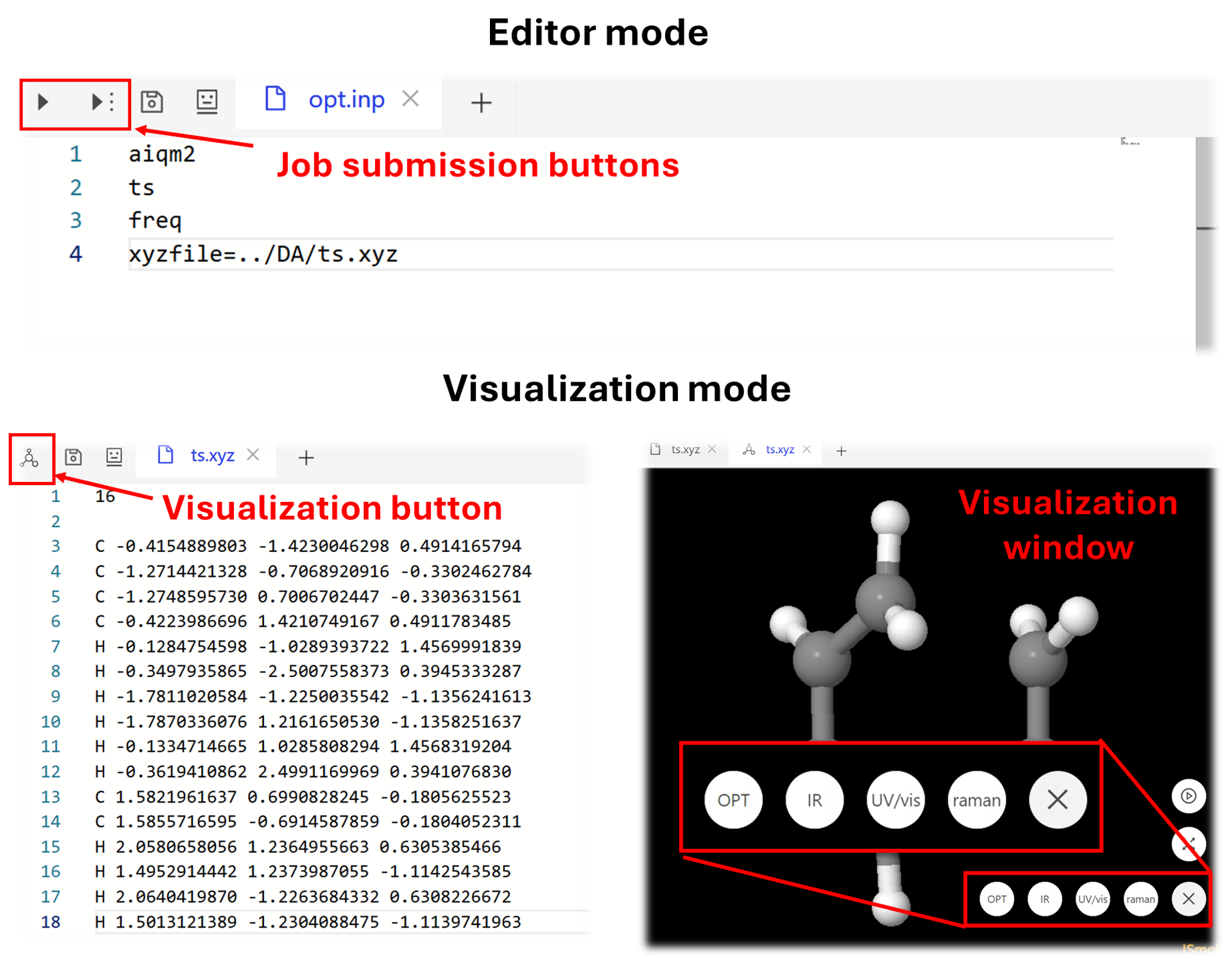
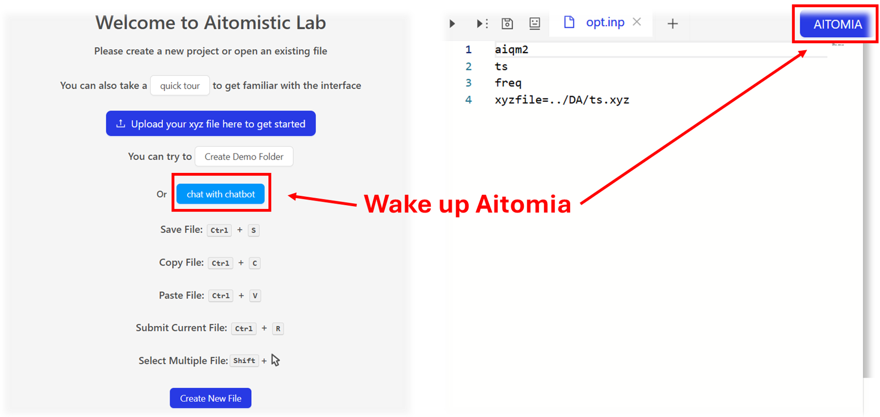
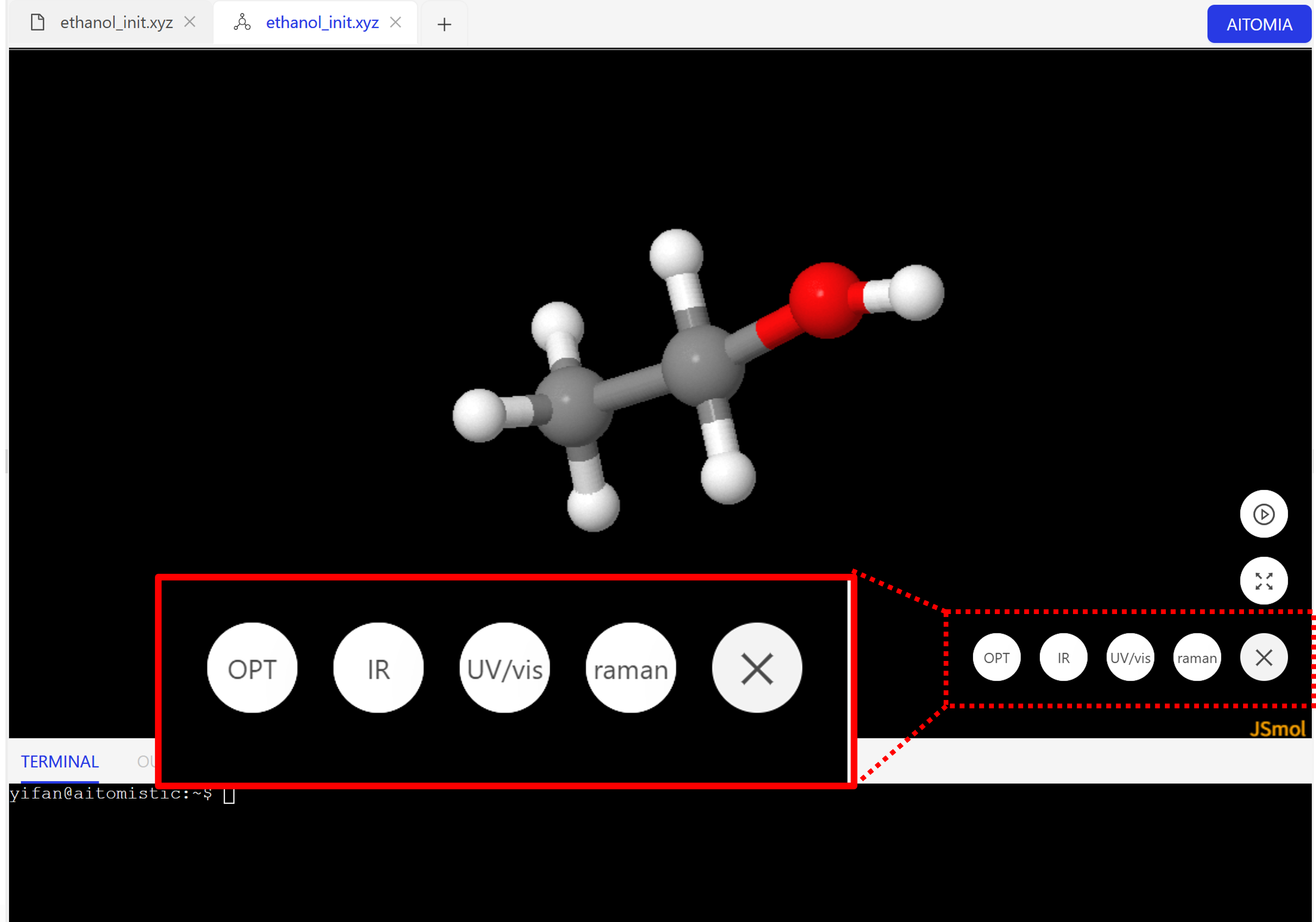
The opened files will be shown in the editor on the right side. You can directly edit the file there as any normal text editor. The input file or the python script for calculation (we will show how to write them later) can be run by clicking the job submission symbol on the upper left corner. If you open a structure file of molecule (currently only .xyz format is supported), you can directly visualize it by clicking the molecule button on the left corner. There are also some options in the visualization window for you to explore, e.g., the opt and ir.

The Chat panel with our intelligent assistant Aitomia can be waken up by clicking chat with chatbot on the welcome page or the AITOMIA on the upper right corner. We will also show later the fully autonomous derivation of the reaction properties by Aitomia.

Explore Diels-Alder reactions with AIQM2

In this section, we will show step by step on Aitomistic Hub, how to find the transition state (TS) of the typical Diels-Alder reaction with AIQM2:

Here, we provide some tutorials to guide you through the whole procedure.

Step 1: Visualize the initial structure

With the above simple introduction to Aitomistic Hub, let’s now use AIQM2 to explore the Diels-Alder reaction. We have provided the initial transition state structure below:

16
ts.xyz
C -0.4154889803 -1.4230046298 0.4914165794
C -1.2714421328 -0.7068920916 -0.3302462784
C -1.2748595730 0.7006702447 -0.3303631561
C -0.4223986696 1.4210749167 0.4911783485
H -0.1284754598 -1.0289393722 1.4569991839
H -0.3497935865 -2.5007558373 0.3945333287
H -1.7811020584 -1.2250035542 -1.1356241613
H -1.7870336076 1.2161650530 -1.1358251637
H -0.1334714665 1.0285808294 1.4568319204
H -0.3619410862 2.4991169969 0.3941076830
C 1.5821961637 0.6990828245 -0.1805625523
C 1.5855716595 -0.6914587859 -0.1804052311
H 2.0580658056 1.2364955663 0.6305385466
H 1.4952914442 1.2373987055 -1.1142543585
H 2.0640419870 -1.2263684332 0.6308226672
H 1.5013121389 -1.2304088475 -1.1139741963

You can try to use the above instructions to visualize it in the visualization panel.

Step 2: TS optimization and frequency calculation

There are two ways to use AIQM2. The easiest way is to create input file like most computational softwares. In our case, we can use input file opt.inp like this:

aiqm2
ts
freq
xyzfile=ts.xyz

The first line AIQM2 tells we want to use AIQM2 to do calculation. ts and freq keywords tells that we will perform transition state geometry optimization and then frequency calculation. xyzfile is used to pass your structure information to MLatom.

The advanced way to use AIQM2 is through python script, where you have more control of the behaviour of AIQM2. You can create a file named opt.py as follows:

import mlatom as ml

# load molecule from xyz file
mol = ml.data.molecule.from_xyz_file('ts.xyz')
# define method
aiqm2 = ml.models.methods(method='AIQM2')

# perform geometry optimization
geomopt = ml.optimize_geometry(
    model = aiqm2,
    initial_molecule = mol,
    ts = True
)

# save optimized geometry
optmol = geomopt.optimized_molecule
optmol.dump('ts_opt.json',format='json')
optmol.write_file_with_xyz_coordinates('optgeoms.xyz')

# perfrom frequency calculation
ml.freq(
    model = aiqm2,
    molecule = optmol
)

# print
print('Frequencies: \n')
print(optmol.frequencies)

Note

The detailed tutorial about using MLatom for geometry optimization can be found here and frequency calculations here. We also have dedicated section for transtion state.

After creating the input file or the python script, you can submit the job by clicking the job submission button. The pumped out terminal space will show the status of the job. You can also check the Job List page:

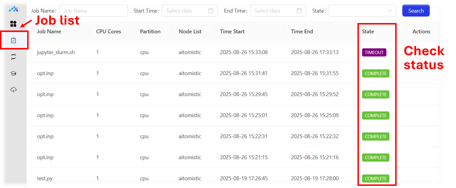
Once the calculation is complete, you may find many files under your current working directory. We will gradually remove these files in the future for easier checking. For now, the optimized geometry can be found in optgeoms.xyz. As usual, you can visualize it with visualization button. Any job will produce output file and the name of the output file is in format [job name].[jobid].out.

Step 3: Visualization of the normal modes

If you use input file, you will find freq_gaussian1.log file. With it, you can visualize the normal modes and frequencies with Chemcraft. Generating log files that are readable for other visualization software is on the todo list.

Another way to visualize the normal modes is via Jupyter Lab.

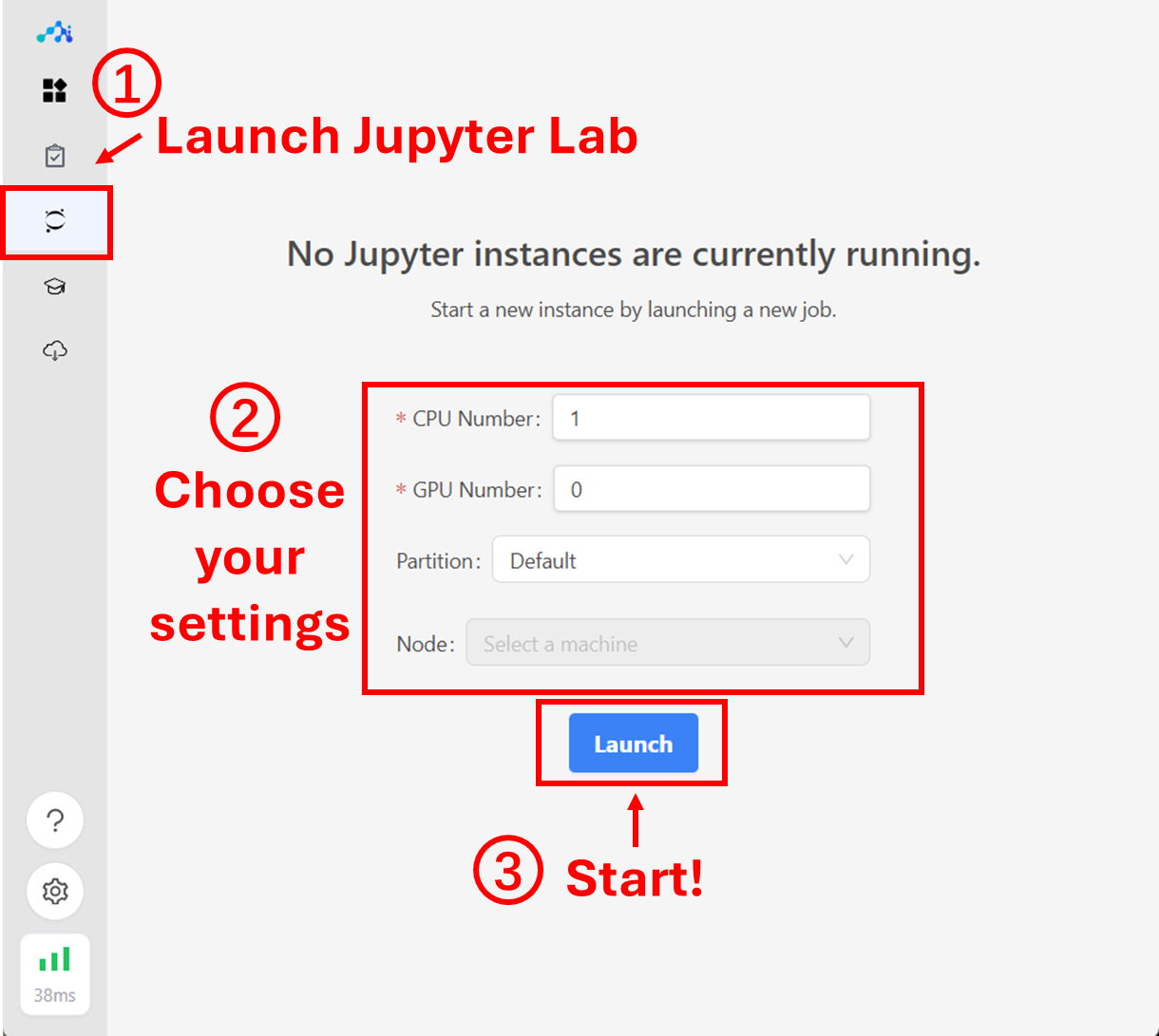
With the opened Jyputer Lab, you can create a new Jupyter notebook under your working directory and execute the Python script cell by cell. The file you will use here is the generated freq1.json file which contains the frequencies and normal modes calculated by AIQM2. We provide the example Jupyter notebook here:

vis

In [1]:

import mlatom as ml

In [2]:

mol = ml.data.molecule.load('freq1.json', format='json')

In [3]:

mol.view()

3Dmol.js failed to load for some reason. Please check your browser console for error messages.

In [5]:

mol.view(normal_mode=0)

3Dmol.js failed to load for some reason. Please check your browser console for error messages.

In [ ]:

To explore more capabilities of visualization with MLatom, Please check our tutorial on frequency visualization

Set charges and multiplicities for your molecules

If molecules have other than default charges (default 0) and multiplicities (default 1), the input might look like:

AIQM2
xyzfile=sp.xyz
charges=0,1
multiplicities=1,3

As you have notice, you can set charges and multiplicities for multiple molecules with comma as the delimiter.

For Python script, each molecule object has charge and multiplicity as their properties. You can derictly change them by using:

import mlatom as ml

mol = ml.data.molecule.from_xyz_file('sp.xyz')
mol.charge = 1
mol.multiplicity = 3

If you load a bunch of molecules as the molecular database, you can pass into an array of values:

import mlatom as ml

moldb = ml.data.molecular_database.from_xyz_file('sp.xyz')
mol.charges = [0, 1]
mol.multiplicity = [1, 3]

Reactive molecular dynamics with AIQM2

This part resembles that in UAIQM tutorial where AIQM2 is selected from the library based on the requested time budget.

IR spectrum with AIQM2

AIQM2 uses its baseline GFN2-xTB to get dipole moment and its derivatives for generating IR spectrum. You can find the detailed tutorial here. The basic usage via input file follows:

ir
AIQM2
xyzfile=opt.xyz

On Aitomistic Hub, you can easily generate the IR spectrum by simply clicking the button on the visualization page

Implicit solvent in AIQM2

Implicit solvent is applied by using keyword baseline_kwargs when defining the method. It can only be used via python script. The available solvents can be found here.

import mlatom as ml

aiqm2 = ml.model.methods(
    method='AIQM2',
    baseline_kwargs={'solvent':'water'})

Convergence problem

Because AIQM2 use GFN2-xTB as baseline, sometimes, you might get the convergence error like this:

[ERROR] Program stopped due to fatal error
-3- Single point calculation terminated
-2- xtb_calculator_singlepoint: Electronic structure method terminated
-1- scf: Self consistent charge iterator did not converge

There are two solutions based on its official documentation. Currently only Python script is supported to change its behavior. And you can pass the additional keywords to GFN2-xTB with:

import mlatom as ml

aiqm2 = ml.model.methods(
    method='AIQM2',
    baseline_kwargs={'read_keywords_from_file':'xtbkw'})

Here, the baseline GFN2-xTB in AIQM2 will read keywords from the file xtbkw. The available keywords can be found in https://github.com/grimme-lab/xtb/blob/main/man/xtb.1.adoc.

Option 1: change the electron temperature

For the theory behind, you can find it https://xtb-docs.readthedocs.io/en/latest/sp.html#fermi-smearing. By default, the electron temperature is 300K.

The content of xtbkw looks like:

--etemp 1000

Option 2: change the SCF convergence criterion

By default, the convergence criterion is set to 10e-6 Hartree, which equals to 1 in keyword --acc. You can change the default accuracy by modifying content of xtbkw:

--acc 10

which means the criterion is set to 10e-5.

Citations

If you have used AIQM2, then the following citations are appropriate in your publication:

Yuxinxin Chen, Pavlo O. Dral*. AIQM2: Organic Reaction Simulations Beyond DFT. Chem. Sci. 2025, accepted manuscript. DOI: 10.1039/D5SC02802G.
IR spectra with AIQM2: Yi-Fan Hou, Cheng Wang, Pavlo O. Dral*. Accurate and Affordable Simulation of Molecular Infrared Spectra with AIQM Models. J. Phys. Chem. A 2025, 129, 3613–3623. DOI: 10.1021/acs.jpca.5c00146.
MLatom: Pavlo O. Dral, Fuchun Ge, Yi-Fan Hou, Peikun Zheng, Yuxinxin Chen, Mario Barbatti, Olexandr Isayev, Cheng Wang, Bao-Xin Xue, Max Pinheiro Jr, Yuming Su, Yiheng Dai, Yangtao Chen, Lina Zhang, Shuang Zhang, Arif Ullah, Quanhao Zhang, Yanchi Ou. MLatom 3: A Platform for Machine Learning-enhanced Computational Chemistry Simulations and Workflows. J. Chem. Theory Comput. 2024, 20, 1193–1213. DOI: 10.1021/acs.jctc.3c01203.
MLatom: Pavlo O. Dral, Fuchun Ge, Yi-Fan Hou, Peikun Zheng, Yuxinxin Chen, Bao-Xin Xue, Max Pinheiro Jr, Yuming Su, Yiheng Dai, Yangtao Chen, Shuang Zhang, Lina Zhang, Arif Ullah, Quanhao Zhang, Yanchi Ou. MLatom: A Package for Atomistic Simulations with Machine Learning, version [add version number], Xiamen University, Xiamen, China, 2013–2024. MLatom.com.
GFN2-xTB* Hamiltonian: C. Bannwarth, S. Ehlert, S. Grimme, J. Chem. Theory Comput. 2019, 15, 1652–1671.
xtb program: Semiempirical extended tight-binding program package xtb.https://github.com/grimme-lab/xtb.
D4: E. Caldeweyher, C. Bannwarth, S. Grimme, J. Chem. Phys. 2017, 147, 034112.
D4 program: E. Caldeweyher, S. Ehlert, S. Grimme, DFT-D4, Version [check your version], (Mulliken Center for Theoretical Chemistry, University of Bonn, [year])
ANI model: J. S. Smith, O. Isayev, A. E. Roitberg, Chem. Sci. 2017, 8, 3192
TorchANI program: X. Gao, F. Ramezanghorbani, O. Isayev, J. S. Smith, A. E. Roitberg, J. Chem. Inf. Model. 2020, 60, 3408