Absorption and emission spectra
This tutorial shows how to calculate and plot UV/vis spectra via single-point convolution and nuclear-ensemble approach (NEA). ML can be used to increase precision of the NEA spectra at reduced cost.
Aborption spectra
Single-point convolution
Here are the required files:
Jupyter notebook
uvvis_scp.ipynb,experimental UV/vis spectrum of benzene from the NIST database:
benzene_exp.dat,pre-calculated excited-state propoerties:
benzene.json.
import mlatom as ml
# here we demonstrate on an example of benzene molecule how to calculate its UV/vis spectrum via single-point convolution
# load the initial guess for geometry
mol = ml.data.molecule.from_xyz_string('''12

C        0.00000000      1.39110400      0.00000000
C        1.20473100      0.69555200      0.00000000
C        1.20473100     -0.69555200      0.00000000
C       -0.00000000     -1.39110400      0.00000000
C       -1.20473100     -0.69555200     -0.00000000
C       -1.20473100      0.69555200      0.00000000
H        0.00000000      2.47330200      0.00000000
H        2.14194200      1.23665100      0.00000000
H        2.14194200     -1.23665100      0.00000000
H       -0.00000000     -2.47330200      0.00000000
H       -2.14194200     -1.23665100     -0.00000000
H       -2.14194200      1.23665100      0.00000000
''')

# define the method
aiqm1 = ml.models.methods(method='AIQM1')

# optimize the geometry in the ground state (can be done in a different method than used for calculating excited-state properties)
ml.optimize_geometry(molecule=mol, model=aiqm1)
print('Optimized geometry:\n')
print(mol.get_xyz_string())
Optimized geometry:

12

C             0.0000000000000           1.3925401460472           0.0000000000000
C             1.2059751422665           0.6962700730233           0.0000000000000
C             1.2059751422665          -0.6962700730233           0.0000000000000
C            -0.0000000000000          -1.3925401460472           0.0000000000000
C            -1.2059751422665          -0.6962700730233           0.0000000000000
C            -1.2059751422665           0.6962700730233           0.0000000000000
H             0.0000000000000           2.4748778305515           0.0000000000000
H             2.1433070725205           1.2374389152757           0.0000000000000
H             2.1433070725205          -1.2374389152757           0.0000000000000
H            -0.0000000000000          -2.4748778305515           0.0000000000000
H            -2.1433070725205          -1.2374389152757           0.0000000000000
H            -2.1433070725205           1.2374389152757           0.0000000000000
# perform single-point excited-state calculations
aiqm1.predict(molecule=mol,
                nstates=30, # Number of electronic states to calculate
                )
# after all this work, let's dump the molecule so that we can re-use the calculations later if needed:
mol.dump(filename='benzene.json', format='json')
# you can load it later as
# mol = ml.molecule.load(filename='benzene.json', format='json')

# show the excitation energies and oscillator strengths
print(f'Excitation energies in eV: {mol.excitation_energies*ml.constants.hartree2eV}')
print(f'Oscillator strengths: {mol.oscillator_strengths}')
Excitation energies in eV: [5.3710049  5.60304691 6.61331818 6.67385531 6.67385531 6.76922225
 7.08701569 7.08701569 7.09072088 7.09072088 7.19999454 7.33800668
 7.33800668 7.68971288 7.68971288 7.78272969 7.94352801 7.94352801
 8.03701885 8.03701885 8.04044002 8.3125381  8.3125381  8.35760543
 8.49747267 8.51403753 8.51403753 8.52262497 8.52262497]
Oscillator strengths: [0.0, 0.0, 0.0, 0.0, 0.0, 0.001118, 0.0, 0.0, 0.200732, 0.200732, 0.0, 0.0, 0.0, 0.0, 0.0, 0.035603, 2.750769, 2.750769, 0.0, 0.0, 0.0, 0.0, 0.0, 0.0, 0.0, 0.0, 0.0, 0.0, 0.0]
mol = ml.molecule.load(filename='benzene.json', format='json')
# now we can use single-point convolution to obtain UV/vis absorption spectrum from our calculations
spectrum = ml.spectra.uvvis.spc(molecule=mol, band_width=0.3)
# dump spectrum in a text or npy format
spectrum.dump('benzene_spc.txt', format='txt')
# you can load it later as
# spectrum = ml.spectra.uvvis.load('benzene_spc.txt', format='txt')
# quick plot to save the spectrum in a file or check it in the Jupyter notebook
spectrum.plot(filename='UVvis.png')

# it might be useful to use dedicated plotting routines which are more flexible,
# e.g., for showing the slider to interactively modify the broadening width in Jupyter notebook
ml.spectra.plot_uvvis(molecule=mol,
               normalize=True,
               spc=True, band_width=0.06,
               band_width_slider=True, # might want to swith off if not used interactively
               )
interactive(children=(FloatSlider(value=0.06, description='width (eV):', max=0.5, min=0.01, step=0.01), Output…
# more useful might be comparison to experiment
# let's get the experimental spectrum from file (got from NIST, baseline is not removed)
wavelengths = []
cross_section = []
import numpy as np

raw_data = np.loadtxt(f'benzene_exp.dat').T
exp_spectrum = ml.spectra.uvvis(wavelengths_nm=raw_data[0],molar_absorbance=raw_data[1])
ml.spectra.plot_uvvis(spectra=[exp_spectrum],
               molecule=mol,
               normalize=True,
               labels=['experiment', 'theory'],
               shift=True,
               spc=True, band_width=0.06,
               band_width_slider=True,
               filename='UVvis_sp_comparison.png'
               #plotstart=300, plotend=600, # other potentially useful options
               #linespectra=[linespec]
               )
interactive(children=(FloatSlider(value=0.06, description='width (eV):', max=0.5, min=0.01, step=0.01), Output…
Nuclear-ensemble approach
Here are the required files:
- Jupyter notebook: uvvis_nea.ipynb,
- experimental UV/vis spectrum of benzene from the NIST database: benzene_exp.dat,
- pre-calculated excited-state properties for an ensemble: benzene_ensemble.json
import mlatom as ml
# here we demonstrate on an example of benzene molecule how to calculate its UV/vis spectrum via NEA approach
# load the initial guess for geometry
mol = ml.data.molecule.from_xyz_string('''12

C        0.00000000      1.39110400      0.00000000
C        1.20473100      0.69555200      0.00000000
C        1.20473100     -0.69555200      0.00000000
C       -0.00000000     -1.39110400      0.00000000
C       -1.20473100     -0.69555200     -0.00000000
C       -1.20473100      0.69555200      0.00000000
H        0.00000000      2.47330200      0.00000000
H        2.14194200      1.23665100      0.00000000
H        2.14194200     -1.23665100      0.00000000
H       -0.00000000     -2.47330200      0.00000000
H       -2.14194200     -1.23665100     -0.00000000
H       -2.14194200      1.23665100      0.00000000
''')

# define the method
aiqm1 = ml.models.methods(method='AIQM1')

# optimize the geometry in the ground state (can be done in a different method than used for calculating excited-state properties)
ml.optimize_geometry(molecule=mol, model=aiqm1)
print('Optimized geometry:\n')
print(mol.get_xyz_string())
Optimized geometry:

12

C             0.0000000000000           1.3925401460472           0.0000000000000
C             1.2059751422665           0.6962700730233           0.0000000000000
C             1.2059751422665          -0.6962700730233           0.0000000000000
C            -0.0000000000000          -1.3925401460472           0.0000000000000
C            -1.2059751422665          -0.6962700730233           0.0000000000000
C            -1.2059751422665           0.6962700730233           0.0000000000000
H             0.0000000000000           2.4748778305515           0.0000000000000
H             2.1433070725205           1.2374389152757           0.0000000000000
H             2.1433070725205          -1.2374389152757           0.0000000000000
H            -0.0000000000000          -2.4748778305515           0.0000000000000
H            -2.1433070725205          -1.2374389152757           0.0000000000000
H            -2.1433070725205           1.2374389152757           0.0000000000000
# we need to obtain an ensemble of geometries. The easiest way through Wigner sampling, but, e.g., MD can be also done.
# here we show for Wigner sampling that requires the frequency calculations
_ = ml.freq(molecule=mol, model=aiqm1)
# check vibrational modes
mol.view(normal_mode=1)
interactive(children=(IntSlider(value=1, description='mode', max=29), Output()), _dom_classes=('widget-interac…
# perform single-point excited-state calculations for comparison (not needed for NEA)
aiqm1.predict(molecule=mol,
                nstates=30, # Number of electronic states to calculate
                )
# after all this work, let's dump the molecule so that we can re-use the calculations later if needed:
mol.dump(filename='benzene.json', format='json')
# you can load it later as
# mol = ml.molecule.load(filename='benzene.json', format='json')
# get the nuclear ensemble with 100 geometries
ensemble = ml.generate_initial_conditions(molecule=mol,
                                                generation_method='Wigner',
                                                initial_temperature=298,
                                                number_of_initial_conditions=100)
# perform single-point excited-state calculations for the ensemble
aiqm1.predict(molecular_database=ensemble,
              nstates=30, # Number of electronic states to calculate
              )
# after all this work, let's dump the molecule so that we can re-use the calculations later if needed:
ensemble.dump(filename='benzene_ensemble.json', format='json')
# you can load it later as
#ensemble = ml.molecular_database.load(filename='benzene_ensemble.json', format='json')
# we can use NEA to obtain UV/vis absorption spectrum from our calculations
spectrum_nea = ml.spectra.uvvis.nea(molecular_database=ensemble, broadening_width=0.02)
# for comparison, we can use single-point convolution to obtain UV/vis absorption spectrum from our calculations
spectrum_spc = ml.spectra.uvvis.spc(molecule=mol, band_width=0.3)
spectrum_nea.plot('UVvis_NEA.png')

# more useful might be comparison to experiment
# let's get the experimental spectrum from file (got from NIST, baseline is not removed)
wavelengths = []
cross_section = []
import numpy as np

raw_data = np.loadtxt(f'benzene_exp.dat').T
exp_spectrum = ml.spectra.uvvis(wavelengths_nm=raw_data[0],molar_absorbance=raw_data[1])
ml.spectra.plot_uvvis(spectra=[exp_spectrum, spectrum_spc, spectrum_nea],
               molecule=mol,
               normalize=True,
               labels=['experiment', 'NEA', 'SPC'],
               )

ML-NEA
NEA is pretty expensive and, hence, we can use ML to speed up the calculations, e.g., with our ML-NEA approach:
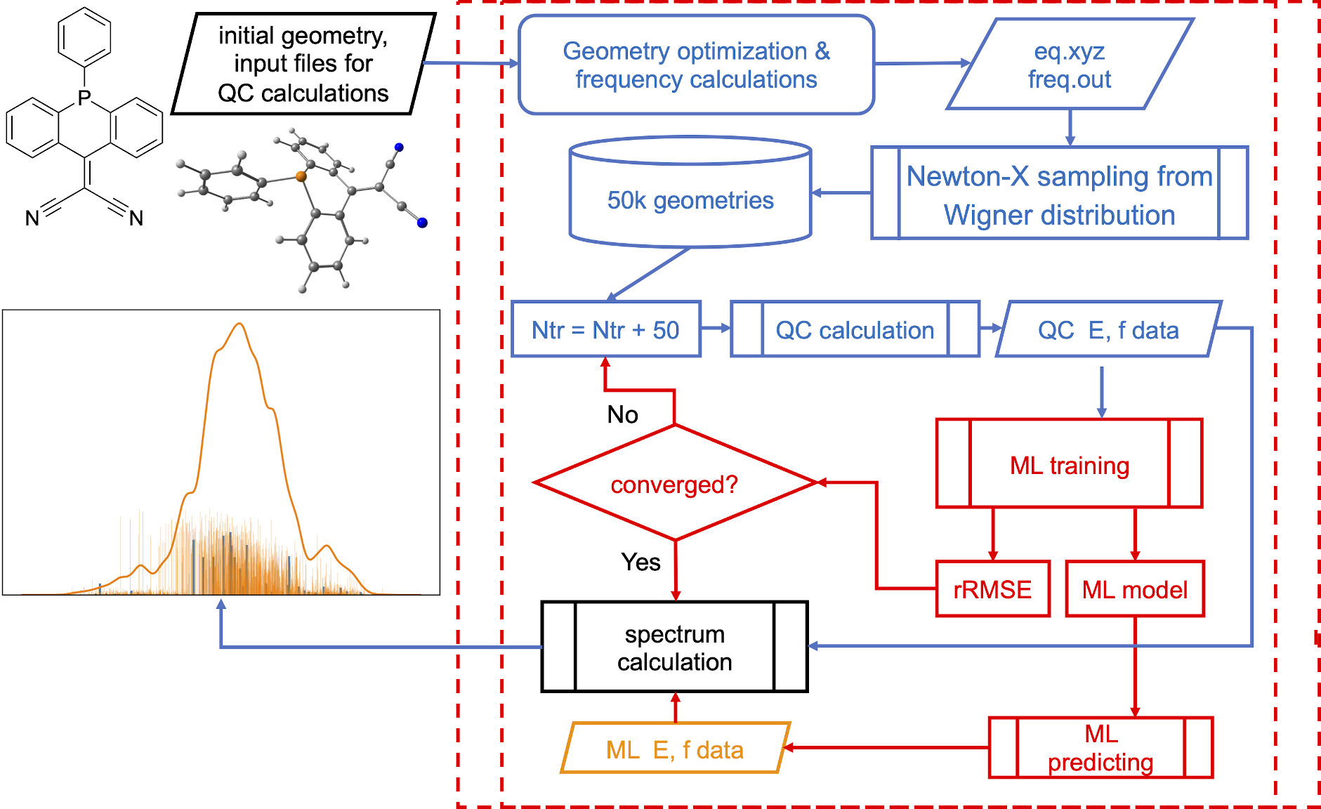
[Credit: Pavlo O. Dral, Fuchun Ge, Bao-Xin Xue, Yi-Fan Hou, Max Pinheiro Jr, Jianxing Huang, Mario Barbatti. MLatom 2: An Integrative Platform for Atomistic Machine Learning. Top. Curr. Chem. 2021, 379, 27. DOI: 10.1007/s41061-021-00339-5, under CC-BY license.]
The following example is based on the precalculated data from our book chapter.
MLatom input file:
cross-section
Nexcitations=30
plotQCNEA
plotQCSPC
deltaQCNEA=0.05
These calculations require many data files (reference excitation energies at TDDFT level).
These data files are zipped. You can upload them as an auxiliary file to the XACS cloud.
Calculations can take more than 5 min. MLatom automatically determines the minimum required number of training points, in this case it needed 200 points for precise spectrum. In the output file you can find that it took 4 iterations to converge:
==========================================================================================
run ML-NEA iteratively for spectrum generation ( ML_train_iter ) started at Wed Dec  1 12:00:19 2021 CST
ML-NEA iteration 1: train_number = 50; RMSE_geom = 0.06717941145022376; rRMSE = 1.0

ML-NEA iteration 2: train_number = 100; RMSE_geom = 0.09043318436728051; rRMSE = 0.25713761026721255

ML-NEA iteration 3: train_number = 150; RMSE_geom = 0.06411060145373663; rRMSE = 0.410580813729204

ML-NEA iteration 4: train_number = 200; RMSE_geom = 0.0695737045717655; rRMSE = 0.07852252732055763

ML-NEA iteration ended after 4 iteration!
run ML-NEA iteratively for spectrum generation ( ML_train_iter ) finished at Wed Dec  1 12:08:01 2021 CST |||| total spent 462.02 sec
==========================================================================================
After the calculations finished, the spectra are plotted to plot.png file in the cross-section sub-directory. It should look like:
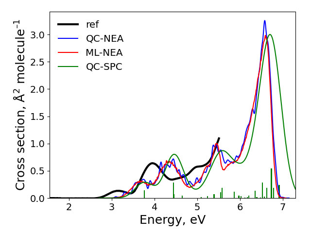
The final result: “ref” is the experimental spectrum, QC-NEA – spectrum calculated with quantum chemical approach on 200 points in ensemble, ML-NEA – machine learning spectrum generated with 200 points in the training set and 50k points in ensemble, QC-SPC – spectrum generated with single-point convolution.
You generate such a spectrum from scratch as described in the manual.
See also a more detailed tutorial.
Emission spectra
Emission spectra simulations are similar to the absorption spectra, with some exceptions. The common technique is optimizing the molecule’s geometry in the first excited state and checking whether the oscillator strengths are high. You can use the single-point convolution, e.g., broaden the peaks with the Gaussian broadening. Geometry optimization requires passing the arguments to the model during the geometry optimizations. These arguments define the number of electronic states to be calculated (including the ground state) and the current state (starts with zero for the ground state).
A code snippet:
# we need to optimize the S1 excited state
# .. request the calculation for the S1 state
#    using the current_state argument passed to the method while making predictions
model_kwargs = {'nstates': 2, 'current_state': 1,
                'calculate_energy_gradients': [True]*2 # required by some methods such as AIQM1 or OM2
                }
ml.optimize_geometry(molecule=mol, model=mymodel, model_predict_kwargs=model_kwargs)
print('Optimized geometry:\n')
print(mol.get_xyz_string())

# show the excitation energies and oscillator strengths
print(f'Excitation energies in eV: {mol.excitation_energies*ml.constants.hartree2eV}')
print(f'Oscillator strengths: {mol.oscillator_strengths}')