User-defined models

Here we show how to create user-defined models with different functions (prediction and training) and of different complexity. See also manual.

Prediction

A typical model is a Python class which has a predict method which accepts molecule and/or molecular_database and has keyword arguments calculate_energy and, often, calculate_energy_gradients. Such a model then needs to add to a molecule or all molecules in the database the required properties (energies and gradients) and can be used for different types of simulations such as single-point calculations, geometry optimization, and molecular dynamics. Here is a Python code snippet to give a better idea:

class mymodel():
    def __init__(self):
        pass

    def predict(self,
        molecule=None,
        molecular_database=None,
        calculate_energy=True,
        calculate_energy_gradients=True
        ):
        if not molecule is None:
            molecule.energy = ... # do required calculations for energy, in Hartree!
            molecule.energy_gradients = ... # in Hartree/Angstrom!
            # Note that energy_gradients = -forces!
        if not molecular_database is None:
            if calculate_energy:
                for mol in molecular_database:
                    mol.energy = ...

model = mymodel()
model.predict(molecule=mymol)
print(mymol.energy)

Note

The model has to use Hartree for energies and Hartree/Angstrom for gradients to be used in many of the simulations, as these units are default in MLatom.

Model trees

Note

Text and figures of this section are adapted from the paper on MLatom 3 in J. Chem. Theory Comput. 2024, DOI: 10.1021/acs.jctc.3c01203 (published under the CC-BY 4.0 license).

Often, it is beneficial to combine several models (not necessarily ML!). One example of such composite models is based on Δ-learning where the low-level QM method is used as a baseline, which is corrected by an ML model to approach the accuracy of the target higher-level QM method. Another example is ensemble learning where multiple ML models are created, and their predictions are averaged during the simulations to obtain more robust results and use in the query-by-committee strategy of active learning. Both of these concepts can also be combined in more complex workflows as exemplified by the AIQM1 method, which uses the NN ensemble as a correcting Δ-learning model and the semiempirical QM method as the baseline. To easily implement these workflows, MLatom allows the construction of the composite models as model trees consisting of model_tree_node, see an example for AIQM1:

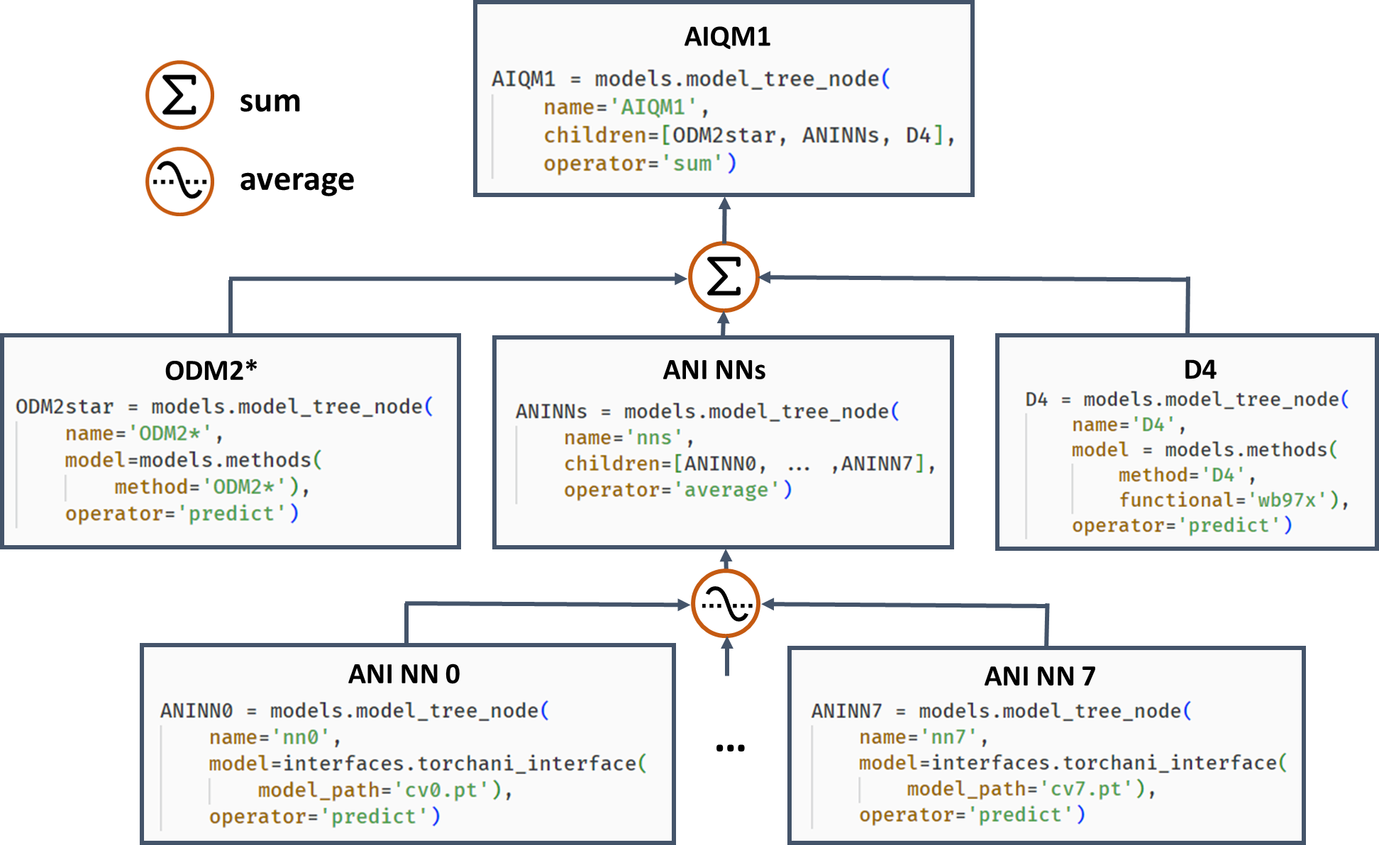
AIQM1’s root parent node comprises three children, the semiempirical QM method ODM2*, the NN ensemble, and additional D4 dispersion correction. The NN ensemble in turn is a parent of eight ANI-type NN children. Predictions of parents are obtained by applying an operation “average” or “sum” to children’s predictions. The code snippets are shown, too.

Other examples of possible composite models are hierarchical ML, which combines several (correcting) ML models trained on (differences between) QM levels, and self-correction, when each next ML model corrects the prediction by the previous model.

Here we show how to use a custom delta-learning model, trained on the differences between full configuration interaction and Hartree–Fock energies.

XYZ coordinates, full CI energies and Hartree–Fock energies of the training points can be downloaded here (xyz_h2_451.dat, E_FCI_451.dat, E_HF_451.dat). You can try to train the delta-learning model by yourself. Here, we provide a pre-trained model delta_FCI-HF_h2.unf.

import mlatom as ml

# Get the initial guess for the molecules to optimize
initmol = ml.data.molecule.from_xyz_file('h2_init.xyz')

# Let's build our own delta-model
# First, define the baseline QM method, e.g.,
baseline = ml.models.model_tree_node(name='baseline',
                                     operator='predict',
                                     model=ml.models.methods(method='HF/STO-3G',
                                                             program='pyscf'))
# Second, define the correcting ML model, in this case the KREG model trained on the differences between full CI and HF
delta_correction = ml.models.model_tree_node(name='delta_correction',
                                             operator='predict',
                                             model=ml.models.kreg(model_file='delta_FCI-HF_h2.unf',
                                                                  ml_program='MLatomF'))
# Third, build the delta-model which would sum up the predictions by the baseline (HF) with the correction from ML
delta_model = ml.models.model_tree_node(name='delta_model',
                                        children=[baseline, delta_correction],
                                        operator='sum')

# Optimize the geometry with the delta-model as usual:
geomopt = ml.optimize_geometry(model=delta_model, initial_molecule=initmol)

# Get the final geometry approximately at the full CI level
final_mol = geomopt.optimized_molecule
print('Optimized coordinates:')
print(final_mol.get_xyz_string())
final_mol.write_file_with_xyz_coordinates(filename='final.xyz')

# Let's check how many full CI calculations, our delta-model saved us
print('Number of optimization steps:', len(geomopt.optimization_trajectory.steps))

This example is inspired by our book chapters on delta-learning and kernel method potentials, with the models trained on data taken from the tutorial book chapter.

Given an initial geometry h2_init.xyz, you will get the following output when using the codes above.

Optimized coordinates:
2

H             0.0000000000000          -0.0000000000000           0.3707890910739
H             0.0000000000000          -0.0000000000000          -0.3707890910739

Number of optimization steps: 4

Training

If you want to write your own ML model architecture and train it on data, you can add train method to your model class. To utilize MLatom’s features, you might want to make use of MLatom’s superclasses which would help to optimize hyperparameters, etc. You would also then have to follow the minimum set of requirements to such a model. First of all, it should accept as keyworded arguments molecular_database (the training set) and property_to_learn=[some string]. Often, models require the validation set, this would need to be provided via validation_molecular_database keyword. property_to_learn can be, e.g., 'energy' or 'y'. Similar, in ML potentials, we want to learn forces if they are available: xyz_derivative_property_to_learn='energy_gradients' would be needed.

Also, after training the model, you probably want to save it somewhere to reuse later. For this, you can specify the model_file while initializing the model class.

A code snippet putting together above considerations:

import mlatom as ml

class mymodel(ml.models.ml_model):
    def __init__(self, model_file=None):
        self.model_file = model_file

    def train(self,
            molecular_database=None,
            validation_molecular_database=None,
            property_to_learn=None,
            xyz_derivative_property_to_learn=None):

        # do the training on molecular database and requested properties
        ...
        # dump the model to disk as specified in self.model_file

Models usually have hyperparameters, they can be added to the model using the special class hyperparameters which consists of class instances of hyperparameters.

For example:

import mlatom as ml

class mymodel(ml.models.ml_model):
    def __init__(self, model_file=None):
        self.hyperparameters = ml.models.hyperparameters({'myhyperparam': ml.models.hyperparameter(value=2**-35,
                                                     minval=2**-35,
                                                     maxval=1.0,
                                                     optimization_space='log',
                                                     name='myhyperparam'),
                            ...})

At the end, your model training may look like:

...
newmodel = mymodel(model_file='newmodel.npz')
newmodel.train(molecular_database=trainDB,
               validation_molecular_database=validateDB,
               property_to_learn='energy',
               xyz_derivative_property_to_learn='energy_gradients'
               )

See examples in the tutorial for ML potentials how to do, e.g., hyperparameter optimization.

Superclasses

In practice, it might be useful to make the model do other operations (e.g., setting the threads, optimizing hyperparameters etc.). Many handy functions like this can be inherited from several common superclasses, with the two most important onces:

• mlatom.models.model – helps to configure multiprocessing, special handling of predictions during geometry optimization (logging the optimization trajectory), etc. This class is strongly recommended to be set as a superclass for your model, e.g., to enable all features in geometry optimizations.

• mlatom.models.ml_model – use it if your model is an ML model which also needs to be trained. This superclass will impart your model with such useful features as hyperparameter optimization, calculation of the validation loss, etc. Note that its superclass is mlatom.models.model, so you do not need to set two of them.

Hence, in practice, you might want to use one of the above superclasses when defining your model:

import mlatom as ml

# for any model
class mymodel(ml.models.model):
    ...
# or for ML models that need to be trained
class mymodel(ml.models.ml_model):
    ...