Delta-learning
Delta-learning is a powerful technique of creating hybrid ML/QM models that have high robustness (stability in simulations), accuracy, and low cost. The delta-learning models are slower than pure ML models but the benefit is typically an increased robustness and accuracy. Delta-learning is the basis of many methods, particularly AIQM1 and UAIQM approaching coupled-cluster accuracy at low cost.
How it works
The key idea behind delta-learning is simple: add ML correction to the predictions of the baseline low-level QM method to approximate the target high-level QM method. Hence, to get a delta-learning model you need to first calculate the target and baseline properties (e.g., energies and forces) for the given data set, find their differences (delta), and train the ML model of your choice (can be any ML potential). Once you have got the model, for a new point, calculate the property with the baseline model and add to it the correction calculated with the ML model.
An example of getting a delta-learning model
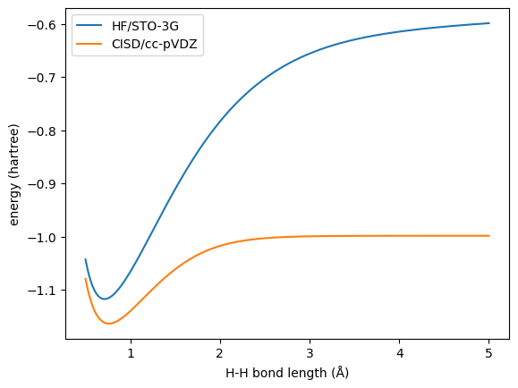
Here we show how to do delta-learning on a simple example of the potential energy curve (PEC) of the hydrogen molecule and we will use the KREG model to learn the correction from the HF/STO-3G to full CI (FCI/cc-pVDZ) level.
See the Jupyter tutorial notebook:
First we need to generate the energies at both baseline and target levels.
import mlatom as ml
import numpy as np
import matplotlib.pyplot as plt

# prepare H2 geometries with bond lengths ranging from 0.5 to 5.0 Å
xyz = np.zeros((451, 2, 3))
xyz[:, 1, 2] = np.arange(0.5, 5.01, 0.01)
z = np.ones((451, 2)).astype(int)
molDB = ml.molecular_database.from_numpy(coordinates=xyz, species=z)

# calculate HF energies
hf = ml.models.methods(method='HF/STO-3G', program='PySCF')
hf.predict(molecular_database=molDB, calculate_energy=True)
molDB.add_scalar_properties(molDB.get_properties('energy'), 'HF_energy') # save HF energy with a new name

# calculate CISD energies
cisd = ml.models.methods(method='CISD/cc-pVDZ', program='PySCF')
cisd.predict(molecular_database=molDB, calculate_energy=True)
molDB.add_scalar_properties(molDB.get_properties('energy'), 'FCI_energy')
Here we use HF/STO-3G as the baseline and CISD/cc-pVDZ (FCI in our case) as the target for the geometries with H–H bond lengths ranging from 0.5 to 5.0 Å.
We need to calculate the differences between the target and baseline:
molDB.add_scalar_properties(molDB.get_properties('FCI_energy') - molDB.get_properties('HF_energy'), 'delta_energy')
Now we can train the KREG model on the differences (basically, residual errors)just on the 12 training points (using 10 sub-training and 2 validation points).
# use every 20th point of the data as the training set and split it into the sub-training and validation sets
step = 20
trainDB = molDB[::step]
val = trainDB[3::5]
sub = ml.molecular_database([mol for mol in trainDB if mol not in val])
# setup the KREG model
kreg = ml.models.kreg(model_file='KREG.npz', ml_program='KREG_API')
# optimize its hyperparameters
kreg.hyperparameters['sigma'].minval = 2**-5 # modify the default lower bound of the hyperparameter sigma
kreg.optimize_hyperparameters(subtraining_molecular_database=sub,
                              validation_molecular_database=val,
                              optimization_algorithm='grid',
                              hyperparameters=['lambda', 'sigma'],
                              training_kwargs={'property_to_learn': 'delta_energy', 'prior': 'mean'},
                              prediction_kwargs={'property_to_predict': 'estimated_delta_energy'})
lmbd = kreg.hyperparameters['lambda'].value ; sigma=kreg.hyperparameters['sigma'].value
valloss = kreg.validation_loss
print('Optimized sigma:', sigma)
print('Optimized lambda:', lmbd)
print('Optimized validation loss:', valloss)
# Train the model with the optimized hyperparameters to dump it to disk.
kreg.train(molecular_database=trainDB, property_to_learn='delta_energy')
After we trained the KREG model, we can use it to estimate the delta corrections for the entire PEC and add them to the baseline predictions to obtain the delta-learning model estimates of the FCI energies:
# predict the delta corrections with the trained KREG model
kreg.predict(molecular_database=molDB, property_to_predict='KREG_delta_energy')
# add them to the baseline values
molDB.add_scalar_properties(molDB.get_properties('HF_energy') + molDB.get_properties('KREG_delta_energy'), 'FCI_energy_est')
Next, let’s train the KREG model directly on the FCI data for comparison and use it for predicting the PEC.
# setup the KREG model
kreg_fci = ml.models.kreg(model_file='KREG.npz', ml_program='KREG_API')
# optimize its hyperparameters
kreg_fci.hyperparameters['sigma'].minval = 2**-5 # modify the default lower bound of the hyperparameter sigma
kreg_fci.optimize_hyperparameters(subtraining_molecular_database=sub,
                                validation_molecular_database=val,
                                optimization_algorithm='grid',
                                hyperparameters=['lambda', 'sigma'],
                                training_kwargs={'property_to_learn': 'FCI_energy', 'prior': 'mean'},
                                prediction_kwargs={'property_to_predict': 'estimated_FCI_energy'})
lmbd = kreg_fci.hyperparameters['lambda'].value ; sigma=kreg_fci.hyperparameters['sigma'].value
valloss = kreg_fci.validation_loss
print('Optimized sigma:', sigma)
print('Optimized lambda:', lmbd)
print('Optimized validation loss:', valloss)
# Train the model with the optimized hyperparameters to dump it to disk.
kreg_fci.train(molecular_database=trainDB, property_to_learn='FCI_energy')
# predict with the direct KREG model
kreg_fci.predict(molecular_database=molDB, property_to_predict='KREG_FCI_energy')
Finally, let’s check the results.
# plot the energies
plt.plot(xyz[:, 1, 2], molDB.get_properties('HF_energy'), label='HF/STO-3G')
plt.plot(xyz[:, 1, 2], molDB.get_properties('FCI_energy'), label='FCI/cc-pVDZ')
plt.plot(xyz[:, 1, 2], molDB.get_properties('FCI_energy_est'), label='delta-learning model')
plt.plot(xyz[:, 1, 2], molDB.get_properties('KREG_FCI_energy'), label='direct KREG')
plt.plot(sub.xyz_coordinates[:, 1, 2], sub.get_properties('FCI_energy'), 'o', label='sub-training points')
plt.plot(val.xyz_coordinates[:, 1, 2], val.get_properties('FCI_energy'), 'o', label='validation points')
plt.legend()
plt.xlabel('H-H bond length (Å)')
plt.ylabel('energy (hartree)')
plt.show()
First, we can see that the delta-learning model trained with all the data has excellent agreement with the reference.
While for the CISD level, the transfer learned model behave way better than the direct one.
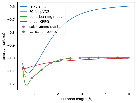
With this example, we can see the power of delta-learning: it provides very robust results even with a small training set. You can compare the performance of this delta-learning model to the analogous exercise with transfer learning.
An example of using delta-learning models in simulations
Here we show how to use a custom delta-learning model, trained on the differences between full configuration interaction and Hartree–Fock energies.
XYZ coordinates, full CI energies and Hartree–Fock energies of the training points can be downloaded here (xyz_h2_451.dat, E_FCI_451.dat, E_HF_451.dat). You can try to train the delta-learning model by yourself. Here, we provide a pre-trained model delta_FCI-HF_h2.unf.
import mlatom as ml

# Get the initial guess for the molecules to optimize
initmol = ml.data.molecule.from_xyz_file('h2_init.xyz')

# Let's build our own delta-model
# First, define the baseline QM method, e.g.,
baseline = ml.models.model_tree_node(name='baseline',
                                     operator='predict',
                                     model=ml.models.methods(method='HF/STO-3G',
                                                             program='pyscf'))
# Second, define the correcting ML model, in this case the KREG model trained on the differences between full CI and HF
delta_correction = ml.models.model_tree_node(name='delta_correction',
                                             operator='predict',
                                             model=ml.models.kreg(model_file='delta_FCI-HF_h2.unf',
                                                                  ml_program='MLatomF'))
# Third, build the delta-model which would sum up the predictions by the baseline (HF) with the correction from ML
delta_model = ml.models.model_tree_node(name='delta_model',
                                        children=[baseline, delta_correction],
                                        operator='sum')

# Optimize the geometry with the delta-model as usual:
geomopt = ml.optimize_geometry(model=delta_model, initial_molecule=initmol)

# Get the final geometry approximately at the full CI level
final_mol = geomopt.optimized_molecule
print('Optimized coordinates:')
print(final_mol.get_xyz_string())
final_mol.write_file_with_xyz_coordinates(filename='final.xyz')

# Let's check how many full CI calculations, our delta-model saved us
print('Number of optimization steps:', len(geomopt.optimization_trajectory.steps))
This example is inspired by our book chapters on delta-learning and kernel method potentials, with the models trained on data taken from the tutorial book chapter.
Given an initial geometry h2_init.xyz, you will get the following output when using the codes above.
Optimized coordinates:
2

H             0.0000000000000          -0.0000000000000           0.3707890910739
H             0.0000000000000          -0.0000000000000          -0.3707890910739

Number of optimization steps: 4