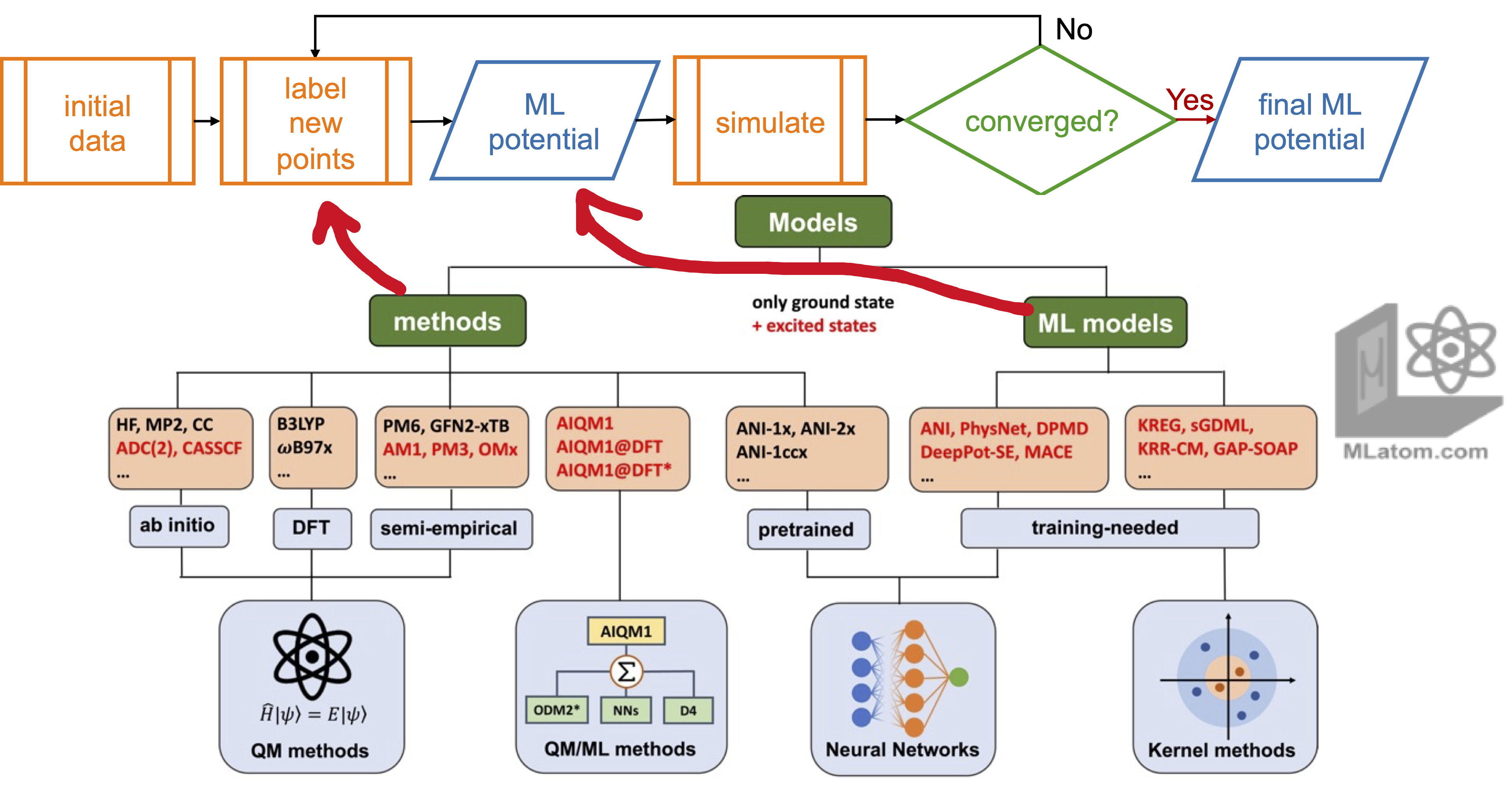
Active learning
Active learning (AL) allows you to collect the data and build ML models required for your application from scratch. In MLatom we provide our physics-informed active learning for efficient building robust ML potentials (MLPs) for molecular dynamics (MD) applications. You can use this procedure with a variety of different MLPs (currently, KREG, ANI, and MACE are supported) and train them on the variety of different QM (DFT, ab initio, …) and even universal ML methods:
Please refer to the following paper for more details (and cite it if you use this procedure):
Yi-Fan Hou, Lina Zhang, Quanhao Zhang, Fuchun Ge, Pavlo O. Dral. Physics-informed active learning for accelerating quantum chemical simulations. 2024, submitted. Preprint on arXiv: https://arxiv.org/abs/2404.11811.
Below we describe how to use AL:
getting started with the minimum setup
distributing labeling on multiple nodes with the queueing system
See the manual for parameters that al function accepts (in Python).
Get started
The minimum setup for active learning with MLatom is very simple as can be seen from the example below of building the ANI potential for the H2 molecule:
AL # request active learning
B3LYP/6-31G* # reference method to label points
# initial guess for the geometry, does not matter much
xyzfile='2

H 0 0 0
H 0 0 0.7'
or in Python API:
import mlatom as ml

h2 = ml.molecule.from_xyz_string('''2

H 0 0 0
H 0 0 0.7
''')

dft = ml.models.methods(method='B3LYP/6-31G*')

ml.al(molecule=h2, reference_method=dft)
Note
Above examples work on the XACS cloud. If you installed MLatom locally, then you need to modify them with method=B3LYP/6-31G* qmprog=pyscf in input file and use dft = ml.models.methods(method='B3LYP/6-31G*', program='PySCF') in Python.
Even for this simple example, it will take looong time on the XACS cloud to finish. Hence, you might want to adjust settings as described below.
import mlatom as ml

h2 = ml.molecule.from_xyz_string('''2

H 0 0 0
H 0 0 0.7
''')

dft = ml.models.methods(method='B3LYP/6-31G*')

# Optimize geometry and calculate frequency
optmol = ml.optimize_geometry(model=dft,initial_molecule=h2).optimized_molecule
freq = ml.freq(model=dft,molecule=optmol)

sampler_kwargs = {
    'initcond_sampler':'wigner',
    'initcond_sampler_kwargs':{'molecule':optmol,'number_of_initial_conditions':100,'initial_temperature':300},
    'maximum_propagation_time':100.0,
    'time_step':0.5,
    'uq_threshold':0.000001,
}

# Start active learning
ml.al(molecule=optmol, ml_model='KREG',sampler_kwargs=sampler_kwargs,min_new_points=5,reference_method=dft)
We provide the Jupyter notebook al.ipynb and h2_freq.json. You can run it after launching the Jupyter lab on the XACS cloud.
al.ipynb and h2_freq.json.
Now, the calculation will take about 15 minutes. The AL will print the progress and at the end will save the final MLP in mlmodel.pt and data in labeled_db.json.
In this example, the AL used the following default settings:
100 quasi-classical MD trajectories at 300 K propagated for 1000 fs.
ANI-type MLP.
training on a GPU if it is available, otherwise on a CPU.
using all threads/CPU cores it can find.
Initial data
Initial data are required to kick start your AL. There are two situations which MLatom can handle:
The user has initial data, which is common if there are some data lying around from the previous projects.
In this case, the user should save the data in MLatom’s
molecular_databaseformat in the fileinit_cond_db.json. This file must be placed in the folder where the AL will be performed.The data has to be created from scratch and dumped in
init_cond_db.jsonfile. This step might be quite slow. Here we cover this situation in more detail.
By default, we use the normal mode (Wigner) sampling to generate the initial data. Also, the reference method used for labeling, is used for geometry optimization and calculation of frequencies and normal modes. The number of initial data points is determined iteratively so that the cross-validation error of ML model would not change by more than 10% after adding additional 50 points based on the learning curve fit (minimum 5 iterations are used for the fit). For judging error, the model is trained only on energies to speed up this step in AL.
The sampling method is defined by parameters initdata_sampler and initdata_sampler_kwargs which are the most important ones you might want to change (see the manual to see how to change other parameters):
ml.al(
    ...
    initdata_sampler=init_dataset_sampler,
    initdata_sampler_kwargs=init_dataset_sampler_kwargs,
    ...
)
The sampler can be either one of the pre-defined functions or the user can create one, see the dedicated instructions. The samplers are common for other steps in active learning procedure, hence, we describe them separately in the dedicated instructions. Here, we briefly overview the key points when using it. Sampler can be, e.g., MD too – particularly if it is affordable to propagate some short trajectories to generate initial data. However, most often you might want to change some of the default settings when doing Wigner sampling of initial data.
For example, often, you can perform the geometry optimizations and frequency calculations in advance, also with a method different from the reference method used for labeling. You might also want to change the temperature. Then the AL script would look like:
optfreq_method = ml.models.methods(method='ANI-1ccx')
eqmol = ml.optimize_geometry(initial_molecule=h2, model=optfreq_method).optimized_molecule
_ = ml.freq(molecule=eqmol, model=optfreq_method)

# or load the molecule with normal modes and frequencies
# eqmol = ml.molecule()
# eqmol.load(filename='eqmol.json', format='json')

init_dataset_sampler = 'wigner'
# or explicitly:
# initial_points_sampler = ml.generate_initial_conditions
init_dataset_sampler_kwargs = {
    #'generation_method': 'Wigner', # required for ml.generate_initial_conditions (although it is default there too)
    'molecule': eqmol,
    'initial_temperature': 500,        # temperature of Wigner sampling in K
    'number_of_initial_conditions': 50 # number of points sampled at one time
}

ml.al(
    ...
    initdata_sampler=init_dataset_sampler,
    initdata_sampler_kwargs=init_dataset_sampler_kwargs,
    ...
)
ML models
By default, MLatom will train the main ANI model on energies and gradients and the auxiliary ANI model only on energies on the entire labeled database generated at this point in AL. This will be used in the physics-informed sampling in each AL iteration.
At the moment, the user can switch from the default ANI to KREG or MACE models with ml_model parameter, e.g.:
ml.al(
    ...
    ml_model = 'KREG',
    ...
)
The user has the flexibility to create their own ML model class for AL. Minimum requirements to such a class:
it must have the usual
trainandpredictfunctions.the
trainfunction must acceptmolecular_databaseparameter.the
predictfunction must acceptmoleculeand/ormolecular_databaseparameters.
Other required parameters can be passed to initialize the ML model with ml_model_kwargs. To summarize, the user defined function and its initialization keywords can be passed to al as:
ml.al(
    ...
    ml_model = my_model,
    ml_model_kwargs = {...},
    ...
)
Hence, any of the MLatoms’ MLPs are acceptable. However, they would be of no use if you do not create the appropriate sampler function to use these MLPs.
See the manual for the fully fledged example of how to create a usable ML model class (used in al routine!).
Sampler
Sampler is one of the key parts of AL as it defines how we collect the points. It is also the one where the user might want to make most adjustments according to their needs. We already encountered sampler in generating initial data. During AL interations, we usually choose a different sampler, i.e., by default we sample by performing 100 quasi-classical MD (1 ps long with 0.1 fs time step) with ML model trained on the previously collected and labelled data, find the the energy deviation to the auxiliary model trained only on energies, stop the MD when the threshold is exceeded, and add this uncertain point to the data set for labeling to start the next iteration.
Hence, the user might want to adjust the settings for performing simulations used to find the points to sample. Example below shows several types of samplers used for different purposes (MD for collecting data and Wigner sampling for generating initial conditions for MD – similar to initial data sampling!):
# let's define our MD for sampling

# ... but before we start, MD needs initial conditions which should always be different, hence, we need another sampler for initial conditions!
md_initconds = 'wigner'
# or explicitly:
# md_initconds = ml.generate_initial_conditions
md_initconds_kwargs = {
    'molecule': eqmol, # must contain normal modes and frequencies!
    #'generation_method': 'Wigner',
    'initial_temperature': 300,        # temperature of Wigner sampling in K
    'number_of_initial_conditions': 100 # defines number of trajectories
}

# ... now we can define our MD sampler
al_sampler = 'md'
# faster and default is batch md, when forces of multiple points in parallel in batches:
#al_sampler = 'batch_md'
sampler_kwargs = {
    'initcond_sampler': md_initconds,
    'initcond_sampler_kwargs': md_initconds_kwargs,
    'maximum_propagation_time':5000.0, # Maximum propagation time; unit: fs
    'time_step':0.5,  # MD time step; unit: fs
}

# Finally, let's pass this info to AL

ml.al(
    ...
    sampler=al_sampler,
    sampler_kwargs=sampler_kwargs,
    ...
)
Sampling function can also be defined by the user. This function must accept ml_model parameter and return molecule_database object with the points to label. Generic example:
def my_sampler(ml_model=None, kwarg1, kwarg2, ...):
    moldb2label = ml.data.molecular_database()
    #do what you need to collect points
    ...
    moldb2label.append(newmol2label)
    return moldb2label

ml.al(
    ...
    sampler=my_sampler,
    sampler_kwargs={kwarg1_with_value, kwarg2_with_value, ...},
    ...
)
In addition, we provide an important option that affects the quality of sampling: uq_threshold. Although it is determined automatically, the user can overwrite it with another number - the smaller the stricter and may lead to many more iterations and sampled points.
Example with these two options (0.5 kcal/mol for the UQ threshold):
ml.al(
    ...
    sampler='md',
    sampler_kwargs={
    'uq_threshold': 0.5/ml.constants.kcalpermol2Hartree,
    ...},
    ...
)
A real example of the sampler function similar to what is used in the physics-informed active learning is given in the manual.
Convergence options
In AL we can control its convergence.
By default, we sample points until 95% of MD trajectories run without encountering a single uncertain prediction. Practically, we run 100 MD trajectories and see whether 5 or more points are still sampled from them - if yes, we repeat the AL cycle. Regardless of sampler, the user can control when AL stops with a keyword min_new_points which request AL to stop when the number of new points sampled in the last iteration is fewer than this parameter.
Another option is new_points which controls the speed of sampling, i.e., the number of new points we would like to sample per each iteration. The default one is None – meaning that the AL will only sample the uncertain points the sampler returns. If it is not None, the AL will attempt to sample more points until it is not fewer than set by new_points. In any case, the AL stops if the min_new_points convergence criterion is met in the first attempt.
Sometimes, we just want to try 1 or couple of AL iterations and stop. For this, the user can use the max_iterations keyword.
Here is a code snippet with an example of using the above keywords:
ml.al(
    ...
    max_iterations = 5,
    new_points     = 300,
    min_new_points = 10,
    ...
)
Other parameters that affect the convergence are the UQ thresholds (uq_threshold), which can be passed as a keyword to sampler.
Distributing labeling on multiple nodes
Generating reference calculations is often slow (that’s why we want to do AL!) and, hence, it is practical to distribute the labeling (calculation of the quantum chemical properties with the reference methods) on multiple computing nodes with the queueing system.
One can do it by writing a wrapper class for the reference method that would handle the distribution with, e.g., crontab or similar tools. We will provide later examples.
Putting it all together
Below is a realistic script for AL for ethanol similar to the protocol we used in publication on physics-informed active learning:
import mlatom as ml

ethanol = ml.molecule.from_xyz_string('''...
''')
eqmol = ml.optimize_geometry(initial_molecule=ethanol, model=optfreq_method).optimized_molecule
_ = ml.freq(molecule=eqmol, model=optfreq_method)

dft = ml.models.methods(method='B3LYP/6-31G*')
init_cond_sampler = 'wigner' # for both initial data and MD
init_dataset_sampler_kwargs = {
    'molecule':eqmol,
    'initial_temperature': 300,
    'number_of_initial_conditions': 50
}
md_initconds_kwargs = {
    'molecule':eqmol,
    'initial_temperature': 300,
    'number_of_initial_conditions': 100
} # We want 100 trajectories at each iteration
# ... now we can define our MD sampler
al_sampler = 'batch_md'
sampler_kwargs = {
    'initcond_sampler': init_cond_sampler,
    'initcond_sampler_kwargs': md_initconds_kwargs,
    'maximum_propagation_time':5000.0, # Maximum propagation time; unit: fs
    'time_step':0.5,  # MD time step; unit: fs
}
ml.al(
    molecule=ethanol,
    reference_method=dft,
    initdata_sampler=init_cond_sampler,
    initdata_sampler_kwargs=init_dataset_sampler_kwargs,
    sampler=al_sampler,
    sampler_kwargs=sampler_kwargs,
    new_points = 300,
)
Restarting
S*t Life happens and AL can crash for whatever reason (the node crashed, run out of memory, AI was in a bad mood today, …). Do not panick! You can restart AL very simply. AL dumps all important infromation (models, UQ thresholds, data, etc – unless you heavily modified the default settings…) in the files in the working directory. Hence restarting simply requires you to start the same calculations in the same folder.
Even in the worst cases, usually you at least have the data (the most important in AL!) and even some models. So you can restart AL with the existing data as initial data.
Also, when you restart, you might want to check the al_info.json which has the parameters of AL. You might want to revise them, e.g., change UQ threshold, etc.
Using MLPs in simulations
The goal of active learning is to accelerate the simulations, hence, after all the work we have done, we want to get our simulation results with the obtained ML models. However, in AL we have already done everything needed for simulations because that’s how we sampled points! Hence, the final AL results are the simulation results.
In practice, AL might not save all required intermediate results such as trajectories. Luckily, the sampler is also a simulator, and we can often reuse the AL routines to do the final simulations.
Alternatively, the models can be also used in other required simulations. For example, after we trained the main ANI model on ethanol, we can use it to optimize ethanol geometry like this:
...
# copy or give the path to the model from the final iteration
ani = ml.models.ani(model_file='iteration10/mlmodel.pt')
ml.optimize_geometry(molecule=ethanol, model=ani)
...
Any questions or suggestions?
If you have further questions, criticism, and suggestions, we would be happy to receive them in English or Chinese via email, Slack (preferred), or QQ (135258964). See our contact page for more information on how to subscribe to updates and follow us on social media.