Surface-hopping dynamics
In this tutorial we show how to perform nonadiabatic molecular dynamics (NAMD) and analysis of NAMD trajectories with MLatom. The simulations are only possible through the Python API. MLatom currently supports Tully’s Fewest Switches Surface Hopping (FSSH) and NAC-free Landau–Zener–Belyev–Lebedev (LZBL) surface hopping.
You can run the TSH with MLatom for the following models:
- FSSH:
MRCI or CASSCF through the interface to COLUMBUS
FSSH with any ML models that provides energies, forces and NACs for electronic states of interset.
- LZBL:
MRCI or CASSCF through the interface to COLUMBUS
ADC(2) through the interface to Turbomole
AIQM1/CI
MS-ANI
Any ML models that provides energies and forces for electronic states of interset.
Running NAMD dynamics
See our papers for more details (please also cite it if you use the corresponding features):
FSSH:
Jakub Martinka, Lina Zhang, Yi-Fan Hou, Mikołaj Martyka, Jiří Pittner, Mario Barbatti, and Pavlo O. Dral. A Descriptor Is All You Need: Accurate Machine Learning of Nonadiabatic Coupling Vectors. 2025. Preprint on arXiv: https://arxiv.org/abs/2505.23344 (2025.05.29).
LZBL:
Lina Zhang, Sebastian Pios, Mikołaj Martyka, Fuchun Ge, Yi-Fan Hou, Yuxinxin Chen, Joanna Jankowska, Lipeng Chen, Mario Barbatti, Pavlo O. Dral. MLatom software ecosystem for surface hopping dynamics in Python with quantum mechanical and machine learning methods. J. Chem. Theory Comput. 2024, 20, 5043–5057. DOI: 10.1021/acs.jctc.4c00468. Preprint on arXiv: https://arxiv.org/abs/2404.06189.
ML-NAMD with AIQM1/MRCI
Note
Please refer to the tutorials of how to use ML for NAMD with MS-ANI and do active learning. The tutorial shown here will need some installations required to perform AIQM1 calculations, while NAMD with ML models will need minimum installations and can be performed online.
Here we show how to use AIQM1/MRCI in propagating LZBL surface-hopping dynamics. Please download the tutorial files (namd_aiqm1.zip).
The script below does all the steps from start to finish:
optimizes geometry
runs frequency calculations
samples initial conditions from the Wigner distribution using Newton-X’s routines. Example can be extended to supports filtering by excitation energy window (refer to the manual for more details)
propagates multiple trajectories in parallel (here 16 trajectories for 5 fs with 0.1 fs time step)
saves trajectories in the h5md format
analyzes results by generating the population plots.
Here is the script:
import mlatom as ml

# Load the initial geometry of a molecule
mol = ml.data.molecule()
mol.charge=1
mol.read_from_xyz_file('cnh4+.xyz')

# Define methods
# .. for NAMD
aiqm1 = ml.models.methods(method='AIQM1',
                        qm_program_kwargs={'save_files_in_current_directory': True,
                                            'read_keywords_from_file':'../materials/mndokw'})
# .. for optimization, frequencies and normal mode calculations
method_optfreq = ml.models.methods(method='B3LYP/Def2SVP', program='pyscf')

# Optimize geometry
geomopt = ml.simulations.optimize_geometry(model=method_optfreq,
                                        initial_molecule=mol)
eqmol = geomopt.optimized_molecule
eqmol.write_file_with_xyz_coordinates('eq.xyz')

# Get frequencies
ml.simulations.freq(model=method_optfreq,
                    molecule=eqmol)
eqmol.dump(filename='eqmol.json', format='json')

# Get initial conditions
init_cond_db = ml.generate_initial_conditions(molecule=eqmol,
                                    generation_method='wigner',
                                    number_of_initial_conditions=16,
                                    initial_temperature=0,
                                    random_seed=1) # To ensure we always get the same initial conditions (should not be used in actual calculations)
init_cond_db.dump('test.json','json')

# Propagate multiple LZBL surface-hopping trajectories in parallel
# .. setup dynamics calculations
namd_kwargs = {
            'model': aiqm1,
            'time_step': 0.25,
            'maximum_propagation_time': 5,
            'hopping_algorithm': 'LZBL',
            'nstates': 3,
            'initial_state': 2, # Numbering of states starts from 0!
            'random_seed': 1 # To ensure we always get the same initial conditions (should not be used in actual calculations)
            }

# .. run trajectories in parallel
dyns = ml.simulations.run_in_parallel(molecular_database=init_cond_db,
                                      task=ml.namd.surface_hopping_md,
                                      task_kwargs=namd_kwargs,
                                      create_and_keep_temp_directories=True)
trajs = [d.molecular_trajectory for d in dyns]

# Dump the trajectories
itraj=0
for traj in trajs:
    itraj+=1
    traj.dump(filename=f"traj{itraj}.h5",format='h5md')

# Analyze the result of trajectories and make the population plot
ml.namd.analyze_trajs(trajectories=trajs, maximum_propagation_time=5)
ml.namd.plot_population(trajectories=trajs, time_step=0.25,
                        max_propagation_time=5, nstates=3, filename=f'pop.png', pop_filename='pop.txt')
And here is the final population plot (your plot will be different because of the random seed in initial conditions and hoppings):

You will also get the text file with populations pop.txt which should look like:
0.000 0.0 0.0 1.0
0.250 0.0 0.0 1.0
0.500 0.0 0.0 1.0
0.750 0.0 0.0 1.0
...
Download the full file cnh4+_aiqm1cis_lznamd_population.txt.
Multi-state ANI models
Multi-state learning model (MS-ANI) that has unrivaled accuracy for excited state properties (accuracy is often better than for models targeting only ground state!). We demonstrate that this model can be used for trajectory-surface hopping of multiple molecules (not just for a single molecule!) in:
Mikołaj Martyka, Lina Zhang, Fuchun Ge, Yi-Fan Hou, Joanna Jankowska, Mario Barbatti, Pavlo O. Dral. Charting electronic-state manifolds across molecules with multi-state learning and gap-driven dynamics via efficient and robust active learning. 2024. Preprint on ChemRxiv: https://doi.org/10.26434/chemrxiv-2024-dtc1w.
Zip with tutorial materials including Jupyter notebook:
#Import MLatom as a Python package.
import mlatom as ml
#First, we define a MS-ANI model
model = ml.models.msani(model_file='fulvene_tutorial.npz',nstates=2)
the trained MS-ANI model will be saved in fulvene_tutorial.npz
#then, we load the training data as a MLatom molecular database. This is a small dataset for
#demo purposes.
train_data = ml.data.molecular_database.load("tutorial_data.json", format="json")
#Now we can train the model.
model.train(molecular_database=train_data,
            property_to_learn='energy',
            xyz_derivative_property_to_learn='energy_gradients',
            hyperparameters={'max_epochs': 100}) #100 epochs is not enough, only for demo.
#The model can be used to make single-point predictions
#First we need to load a fulvene molecule from .xyz
mol = ml.data.molecule()
mol.read_from_xyz_file('fulvene.xyz')
mol.view()
3Dmol.js failed to load for some reason. Please check your browser console for error messages.
#Now we can make a prediction
model.predict(molecule=mol, nstates=2, current_state=0,
              calculate_energy=True, calculate_energy_gradients=True)

#And print the results
for state in mol.electronic_states:
    print(state.energy)
gap = (mol.electronic_states[1].energy-mol.electronic_states[0].energy)*ml.constants.Hartree2eV
print("The S1-S0 gap is {} eV".format(gap))
-230.56873760870891
-230.49484480298358
The S1-S0 gap is 2.010727281361726 eV
#Finally, we can use the MS-ANI model to run NAMD.
#For that we will load a model trained in the AL loop.
model_namd = ml.models.msani(model_file='fulvene_energy_iteration_19.npz')
model loaded from fulvene_energy_iteration_19.npz
#Load an initial conditions database
init_db = ml.data.molecular_database.load("init_cond_db.json", format="json")
#And define NAMD arguments
timemax = 60 # fs
namd_kwargs = {
            'model': model_namd,
            'time_step': 0.1, # fs
            'maximum_propagation_time': timemax,
            'hopping_algorithm': 'LZBL',
            'nstates': 2,
            'reduce_kinetic_energy': True,
            }
#And finally run the NAMD. This should take about a minute.
dyns = ml.simulations.run_in_parallel(molecular_database=init_db[:4], task=ml.namd.surface_hopping_md, task_kwargs=namd_kwargs, create_and_keep_temp_directories=False)
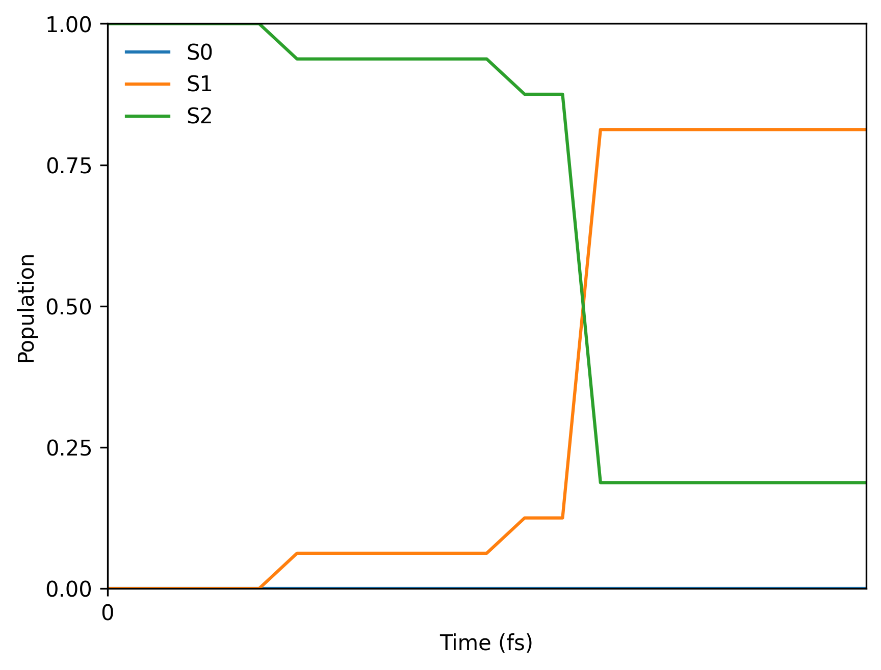
#Now we can plot the results
trajs = [d.molecular_trajectory for d in dyns]
ml.namd.plot_population(trajectories=trajs, time_step=0.1,
                        max_propagation_time=timemax, nstates=2)

#MLatom trajectories can be analyzed and visualized using simple Python code. An example below.
energies = [[],[]]
time = []
gap = []
for step in trajs[0].steps:
    energies[0].append(step.molecule.electronic_states[0].energy)
    energies[1].append(step.molecule.electronic_states[1].energy)
    time.append(step.time)
    gap.append(step.molecule.electronic_states[1].energy-step.molecule.electronic_states[0].energy)
import matplotlib.pyplot as plt
import numpy as np
plt.plot(time, np.transpose(energies))
plt.xlabel("Time (fs)")
plt.ylabel("Energy (Hartree)")
plt.legend(['S0', 'S1'])
<matplotlib.legend.Legend at 0x2adbeae2d940>

ML-NAMD with single-state ML models
In this tutorial, we show an example of running surface-hopping MD with single-state ML models. Please see a separate tutorial on machine learning potentials.
See our paper for more details (please also cite it if you use the corresponding features):
Lina Zhang, Sebastian Pios, Mikołaj Martyka, Fuchun Ge, Yi-Fan Hou, Yuxinxin Chen, Joanna Jankowska, Lipeng Chen, Mario Barbatti, Pavlo O. Dral. MLatom software ecosystem for surface hopping dynamics in Python with quantum mechanical and machine learning methods. J. Chem. Theory Comput. 2024, 20, 5043–5057. DOI: 10.1021/acs.jctc.4c00468. Preprint on arXiv: https://arxiv.org/abs/2404.06189.
You can download the Jupyter notebook with the required initial conditions and ML models from this paper.
The tutorial calculations are very fast and you should be able to get the final population plot for 5 fs with 0.25 fs time step from 30 trajectories within a minute. Here is the Jupyter notebook code snippet:
import mlatom as ml
import os
import numpy as np
# Read initial conditions
init_cond_db = ml.data.molecular_database.load(filename='materials/init_cond_db_for_pyrazine.json', format='json')
# We need to create a class that accepts the specific arguments shown below and saves the calculated electronic state properties in the molecule object
class mlmodels():
def __init__(self, nstates = 5):
folder_with_models = 'materials/lz_models'
self.models = [None for istate in range(nstates)]
for istate in range(nstates):
self.models[istate] = [ml.models.ani(model_file=f'{folder_with_models}/ensemble{ii+1}s{istate}.pt') for ii in range(2)]
for ii in range(2): self.models[istate][ii].nthreads = 1
def predict(self,
molecule=None,
nstates=5,
current_state=0,
calculate_energy=True,
calculate_energy_gradients=True):
molecule.electronic_states = [molecule.copy() for ii in range(nstates)]
for istate in range(nstates):
moltmp = molecule.electronic_states[istate]
moltmpens = [moltmp.copy() for ii in range(2)]
for ii in range(2):
self.models[istate][ii].predict(molecule=moltmpens[ii], calculate_energy = True, calculate_energy_gradients = True)
moltmp.energy = np.mean([moltmpens[ii].energy for ii in range(2)])
moltmp.energy_gradients = np.mean([moltmpens[ii].energy_gradients for ii in range(2)], axis=0)
molecule.energy = molecule.electronic_states[current_state].energy
molecule.energy_gradients = molecule.electronic_states[current_state].energy_gradients
models = mlmodels()
# Arguments for running NAMD trajectories
timemax = 5 # fs
namd_kwargs = {
'model': models,
'time_step': 0.25, # fs
'maximum_propagation_time': timemax,
'dump_trajectory_interval': None,
'hopping_algorithm': 'LZBL',
'nstates': 5,
'random_seed': 1, # making sure that the hopping probabilities are the same (should not be used in actual calculations!)
'rescale_velocity_direction': 'along velocities',
'reduce_kinetic_energy': False,
}
# Run 30 trajectories
dyns = ml.simulations.run_in_parallel(molecular_database=init_cond_db[:30], task=ml.namd.surface_hopping_md, task_kwargs=namd_kwargs)
trajs = [d.molecular_trajectory for d in dyns]
ml.namd.analyze_trajs(trajectories=trajs, maximum_propagation_time=timemax)
# Dump the trajectories
for itraj in range(len(trajs)):
trajs[itraj].dump(filename=f'traj{itraj+1}.json', format='json')
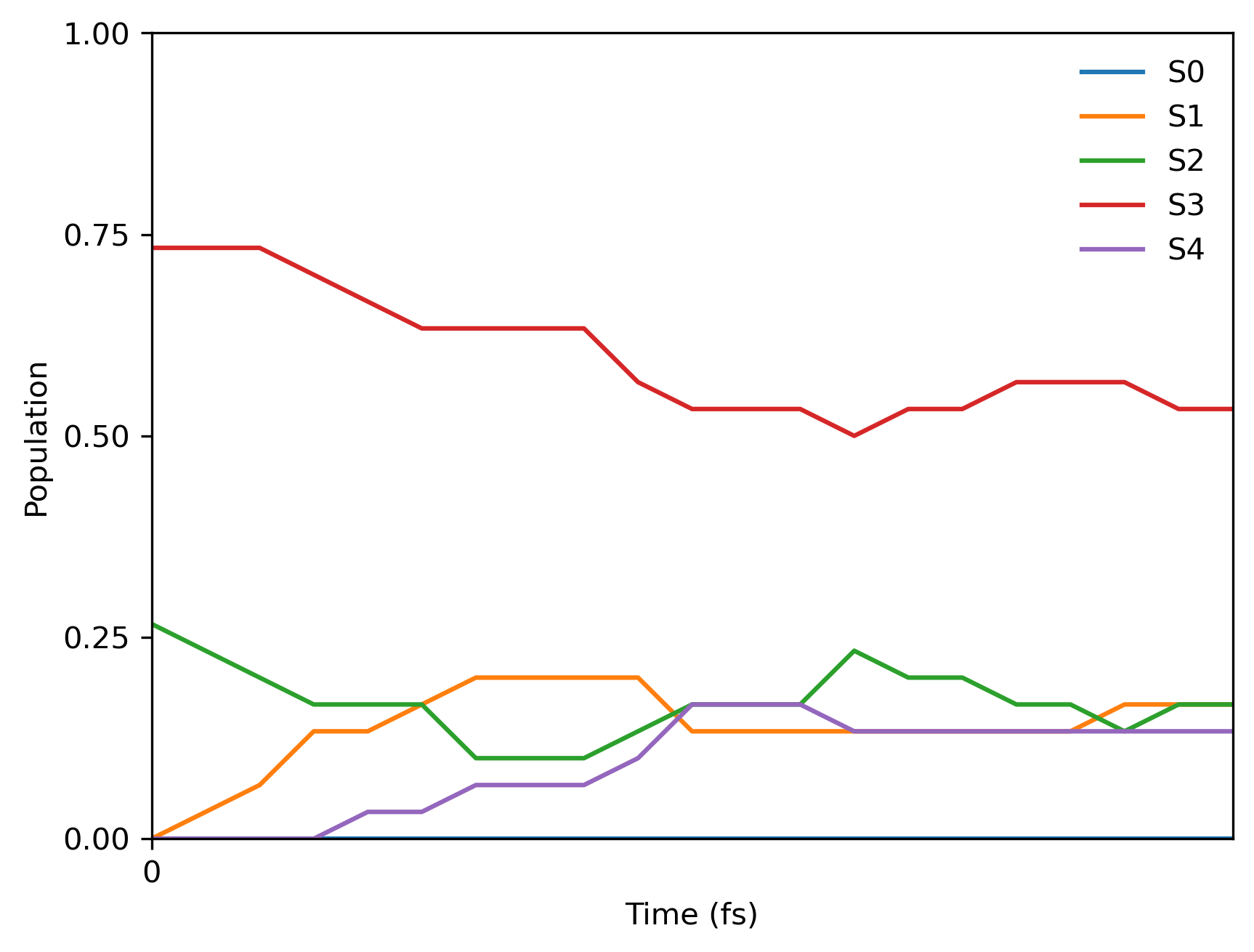
# Prepare the population plot
ml.namd.plot_population(trajectories=trajs, time_step=0.25,
max_propagation_time=timemax, nstates=5, filename=f'pop.png')
Since we used the fixed random seed, you should get the following final population:
FSSH with Columbus
Here we show how to use MRCI (or CASSCF) in propagating Tully’s FSSH dynamics. Please download the tutorial files (fssh_col.zip).
The script only demonstrate possible keywords for performing FSSH:
import mlatom as ml
import matplotlib.pyplot as plt

# Firstly we load an initial conditions
init_cond_db = ml.data.molecular_database.load('test.json','json')

# Define Columbus, this requires to prepare Columbus inputs into 'columbus' directory
col = ml.models.methods(program='columbus',
                        command_line_arguments=['-m', '1700'],
                        directory_with_input_files=f'columbus',
                        save_files_in_current_directory=False)

# Propagate multiple FSSH trajectories in parallel
# .. setup dynamics calculations
namd_kwargs = {
            'model': col,
            'model_predict_kwargs': {'level_of_theory': 'MRCI'}, # Default is CASSCF
            'time_step': 0.25,
            'time_step_tdse': 0.0125, # default value is time_step/20
            'maximum_propagation_time': 5,
            'hopping_algorithm': 'FSSH', # model has to provide nonadiabatic coupling vectors
            'integrator': 'Butcher', # Runge-Kutta 4th order 'RK4' is available as well
            'decoherence_model': 'SDM', # Decoherence correction type: Simplified decay of mixing
            'decoherence_SDM_decay': 0.1,
            'rescale_velocity_direction': 'nacv', # Rescaling along NACs
            'nstates': 3,
            'initial_state': 2, # Numbering of states starts from 0!
            'random_seed': 1 # To ensure we always get the same initial conditions (should not be used in actual calculations)
            }

# .. run trajectories in parallel (this will take around 5 minutes)
dyns = ml.simulations.run_in_parallel(molecular_database=init_cond_db,
                                      task=ml.namd.surface_hopping_md,
                                      task_kwargs=namd_kwargs,
                                      create_and_keep_temp_directories=False)
trajs = [d.molecular_trajectory for d in dyns]

# Dump the trajectories
itraj=0
for traj in trajs:
    itraj+=1
    traj.dump(filename=f"traj{itraj}.h5",format='h5md')

# Analyze the result of trajectories and make the population plot
ml.namd.analyze_trajs(trajectories=trajs, maximum_propagation_time=5)
ml.namd.plot_population(trajectories=trajs, time_step=0.25,
                        max_propagation_time=5, nstates=3, filename=f'pop.png', pop_filename='pop.txt')
And here is the final population plot (your plot will be different because of the random seed in initial conditions and hoppings):
You will also get the text file with populations pop.txt which should look like:
0.000 0.0 0.0 1.0
0.250 0.0 0.0 1.0
0.500 0.0 0.0 1.0
0.750 0.0 0.0 1.0
...
Download the full file cnh4+_mrci_fssh_population.txt.
Analyzing results
General analysis of NAMD trajectories
Author: Mikołaj Martyka
This tutorial shows how to analyse results of NAMD simulations and extract data from an ensamble of trajectories. The data used in this tutorial is available at this DOI: 10.6084/m9.figshare.28044863 Taken from our paper on active learning for TSH simulations, available at: https://chemrxiv.org/engage/chemrxiv/article-details/66e7e01712ff75c3a177a270
import mlatom as ml
Example 1: Analysis of the hopping geometries in fulvene
As a first example we will analyse hopping geometries of fulvene, after excitation to S1. Reference, eg. doi.org/10.12688/openreseurope.13624.2
#Define a function for extracting hopping geometries.
def get_hop_geos(traj):
        nstates = len(traj.steps[0].molecule.electronic_states)
        local_hop_list = [[ [] for k in range(nstates)] for j in range(nstates)]
        for index, geom in enumerate(traj.steps):
            if index !=0:
                if geom.current_state != traj.steps[index-1].current_state:
                    hop_to = int(geom.current_state)
                    hop_from = int(traj.steps[index-1].current_state)
                    traj.steps[index-1].molecule.hoptime = traj.steps[index-1].time
                    print
                    local_hop_list[hop_from][hop_to].append(traj.steps[index-1].molecule)

        geoms = []
        for k in range(nstates):
            for j in range(nstates):
                if local_hop_list[k][j] != None:
                    for idx, hop_geom in enumerate(local_hop_list[k][j]):
                        hop_geom.hop_from = k
                        hop_geom.hop_to = j
                        geoms.append(hop_geom)
        return geoms
#Load a fulvene molecule in MLatom format
mol = ml.data.molecule.load("eqmol.json", format='json')
#Check what is the numbering of the atoms in the xyz file
mol.write_file_with_xyz_coordinates("fulvene.xyz")
mol.view()
3Dmol.js failed to load for some reason. Please check your browser console for error messages.
#Define lists for the relevant quantities
C_CH2_lens = [] #The bond length between atoms no. 0 and 5
#The four dihedral angles required for eq. (8)
C_CH2_dihedral_Cis1= []
C_CH2_dihedral_Cis2 = []
C_CH2_dihedral_trans1 = []
C_CH2_dihedral_trans2 = []
#List for hop times
hop_times = []
#Iterate over trajectories...
for i in range(50):
    #...load them...
    traj = ml.data.molecular_trajectory()
    traj.load("traj{}.json".format(i+1), format='json')
    #...extract hop geoms...
    hop_geoms = get_hop_geos(traj)
    #...and finally extract the data.
    for mol in hop_geoms:
        C_CH2_lens.append(mol.bond_length(0, 5))
        C_CH2_dihedral_Cis1.append(mol.dihedral_angle(2, 0, 5,10))
        C_CH2_dihedral_Cis2.append(mol.dihedral_angle(1, 0, 5,11))
        C_CH2_dihedral_trans1.append(mol.dihedral_angle(2, 0, 5,11))
        C_CH2_dihedral_trans2.append(mol.dihedral_angle(1, 0, 5,10))
        hop_times.append(mol.hoptime)
#Calculate the mean dihedral angle according to  Barbatti et al Open. Res. Eur. 2022, 1, 49.
hop_angle = []
for i in range(len(C_CH2_dihedral_Cis1)):
    sum1 = abs(C_CH2_dihedral_Cis1[i])+abs(C_CH2_dihedral_Cis2[i])+abs(180-abs(C_CH2_dihedral_trans1[i]))+abs(180-abs(C_CH2_dihedral_trans2[i]))
    hop_angle.append(0.25*sum1)
import matplotlib.pyplot as plt
#Plot the results, using the hopping times as a colormap. See fig 5 of 10.26434/chemrxiv-2024-dtc1w-v2 for a plot with more points and explanation.
plt.scatter(C_CH2_lens, hop_angle, c=hop_times)
cbar = plt.colorbar()
cbar.set_label('Time (fs)')
plt.xlabel("C=CH2 distance (A)")
plt.ylabel("Mean C=CH2 dihedral (degrees)")
Text(0, 0.5, 'Mean C=CH2 dihedral (degrees)')

Example 2: Analysis of the quantum yield of cis -> trans photoisomerization of azobenzene
Now we will calculate the quantum yield (QY) of azobenzene cis -> trans isomerisation. Reference: 10.26434/chemrxiv-2024-dtc1w-v2, fig. 7 and text.
#list for dihedral angles
dih_fin = []
#Iterate over trajectories
for i in range(50):
    #Load the final geometries of each trajectory. Notice that the format and location is different, this is the typical output of MLatom's run_in_parallel.
    traj = ml.data.molecular_trajectory()
    traj.load("job_surface_hopping_md_{}/traj.h5".format(i+1), format='h5md')
    #Take the final geometry in each trajectory...
    finmol = traj.steps[-1].molecule
    #...and the dihedral angle.
    dih_fin.append(finmol.dihedral_angle(11, 23, 22,3))
#View one representative trajectory
traj.view()
3Dmol.js failed to load for some reason. Please check your browser console for error messages.
#Plot a histogram of the dihedral angles
plt.hist(dih_fin)
plt.ylabel("Count")
plt.xlabel("Dihedral angle (Deg.)")
Text(0.5, 0, 'Dihedral angle (Deg.)')

#Count the number of trans-azobenzenes at the end, taking the descriptor of dihedral >60 as trans-azobenzene.
counter = 0
for angle in dih_fin:
    if angle > 60:
        counter+=1
#Print the QY
QY = counter/50*100
print("The quantum yield is {}%!".format(QY))
The quantum yield is 68.0%!
Analysis of FSSH trajectories
Trajectories resulting from ‘FSSH’ keyword contain information about propagation of state coefficients and other quantities that are interpolated during this process. Here we take a look at the detailed analysis for a single trajectory. It is possible to access those substep quantities:
substep_potential_energy
substep_velocities
substep_nonadiabatic_coupling_vectors
substep_time_derivative_coupling
substep_state_coefficients
substep_state_coefficients_dot
substep_phase
substep_random_numbers
substep_hopping_probabilities
We start with extracting data into dictionary for convenient plotting :
# Due to the stochastic nature fo FSSH, you may need to load
# different trajectory to see hopping
traj = ml.data.molecular_trajectory()
traj.load('traj6.h5', format='h5md')

dt = 0.25
qdt = dt/20

data_ML = {
    'S0': [],
    'S1': [],
    'S2': [],
    'curr': [],
    'time': [],
}

sh_data_ML = {
    'substep': [],
    'pop0': [],
    'pop1': [],
    'pop2': [],
    'pop_tot': [],
    'dtc01': [],
    'dtc02': [],
    'dtc12': [],
}

for istep in range(len(traj.steps)):
    data_ML['time'].append(istep*dt)
    data_ML['S0'].append(traj.steps[istep].molecule.electronic_states[0].energy)
    data_ML['S1'].append(traj.steps[istep].molecule.electronic_states[1].energy)
    data_ML['S2'].append(traj.steps[istep].molecule.electronic_states[2].energy)
    data_ML['curr'].append(traj.steps[istep].molecule.electronic_states[int(traj.steps[istep].current_state)].energy)
    if istep != len(traj.steps)-1:
        # for classical time step at t, the last element is the same as first element of t+dt
        for isubstep in range(len(traj.steps[0].substep_state_coefficients)-1):
            sh_data_ML['substep'].append(istep*dt+isubstep*qdt)
            sh_data_ML['pop0'].append(abs(traj.steps[istep].substep_state_coefficients[isubstep][0])**2)
            sh_data_ML['pop1'].append(abs(traj.steps[istep].substep_state_coefficients[isubstep][1])**2)
            sh_data_ML['pop2'].append(abs(traj.steps[istep].substep_state_coefficients[isubstep][2])**2)
            sh_data_ML['pop_tot'].append(sh_data_ML['pop0'][-1]+sh_data_ML['pop1'][-1]+sh_data_ML['pop2'][-1])
            sh_data_ML['dtc01'].append(traj.steps[istep].substep_time_derivative_coupling[isubstep][0][1])
            sh_data_ML['dtc02'].append(traj.steps[istep].substep_time_derivative_coupling[isubstep][0][2])
            sh_data_ML['dtc12'].append(traj.steps[istep].substep_time_derivative_coupling[isubstep][1][2])
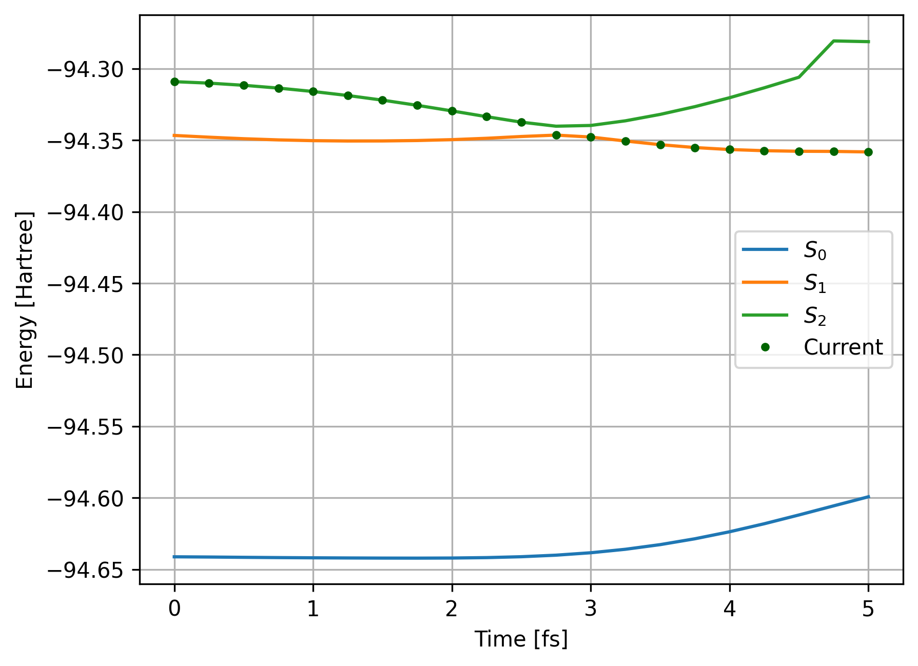
As before, we can plot the energetical profile of trajectory:
fig, ax = plt.subplots()

ax.set_xlabel("Time [fs]")
ax.set_ylabel("Energy [Hartree]")

ax.plot(data_ML['time'], data_ML['S0'], label="$S_0$")
ax.plot(data_ML['time'], data_ML['S1'], label="$S_1$")
ax.plot(data_ML['time'], data_ML['S2'], label="$S_2$")
ax.plot(data_ML['time'], data_ML['curr'], "o", color='darkgreen', markersize=3, label="Current")

ax.grid()
ax.legend()
plt.show()
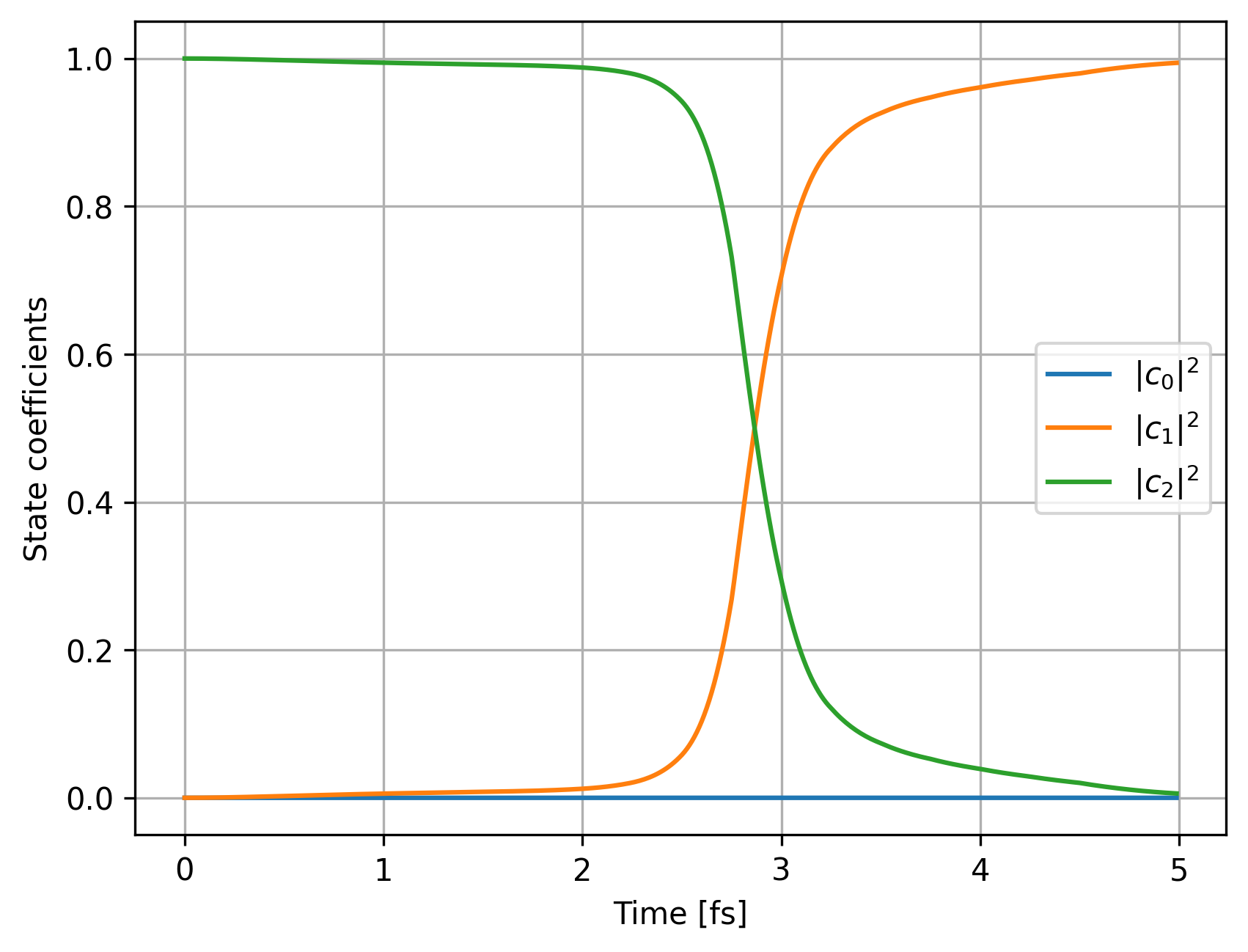
With FSSH, we can check the evolution of state coefficients:
fig, ax1 = plt.subplots()

ax.set_xlabel("Time [fs]")
ax.set_ylabel("State coefficients")

ax.plot(sh_data_ML['substep'], sh_data_ML['pop0'], label="$|c_0|^2$")
ax.plot(sh_data_ML['substep'], sh_data_ML['pop1'], label="$|c_1|^2$")
ax.plot(sh_data_ML['substep'], sh_data_ML['pop2'], label="$|c_2|^2$")

ax.grid()
ax.legend()
ax.show()
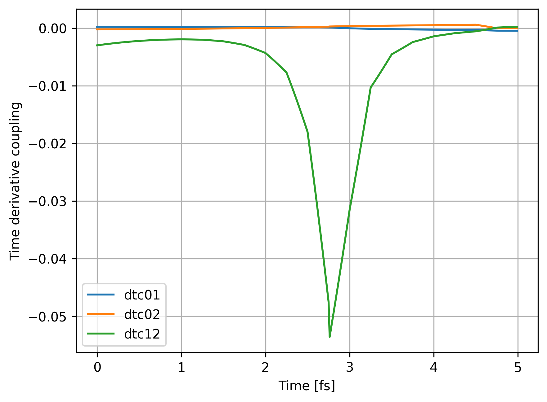
We can take a look how time derivative coupling changed:
fig, ax = plt.subplots()

ax.set_xlabel("Time [fs]")
ax.set_ylabel("Time derivative coupling")

ax.plot(sh_data_ML['substep'], sh_data_ML['dtc01'], label="dtc01")
ax.plot(sh_data_ML['substep'], sh_data_ML['dtc02'], label="dtc02")
ax.plot(sh_data_ML['substep'], sh_data_ML['dtc12'], label="dtc12")

ax.grid()
ax.legend()
ax.show()