Machine learning potentials
This tutorial contains:
overview of MLPs supported by MLatom
explanations how to
use MLPs in simulations
dedicated tutorials for specific types of MLPs:
how to benchmark MLPs and choose the best for your application
For examples how to train, test, and use ML potentials (MLPs) you can see tutorials below. In addition, you can check the command-line and Python API manuals. For these examples, the materials are available as zip archive. It contains Jupyter notebook tutorial_mlp.ipynb. After uploading the content of the zipped directory to the XACS cloud, you can run it on XACS Jupyter lab. For a fast training speed, here we use a 451-point dataset for H2 with H–H bond length ranging from 0.5 to 5.0 Å. The dataset is randomly splitted into a training set of 361 points (H2.xyz, H2_HF.en, H2_HF.grad, which store the geometries, potential energies, and energy gradients, respectively) and a test set of 90 points (names begin with “test_”).
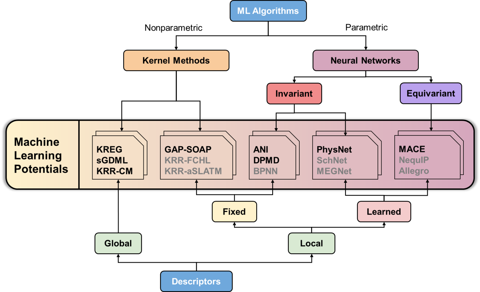
Supported MLPs
The overview of MLPs supported by MLatom (in bold) and other representatives (modified from our MLP benchmark paper):
Note
The fastest potentials to train on small data in this tutorial is to use the kernel models such as KREG model or sGDML. Slower options might be more accurate for your application and more data. For example, ANI has a great cost/performance ratio, but if you have enough resources, you can use very slow MACE which was shown to outperform most of other MLPs. In general, you need to benchmark them on your data and application.
Prerequisites
You can run the examples on the XACS cloud. Otherwise, you might need to install the required packages for MLPs.
For the KREG model through the KREG_API program, the following commands for installing packages might be required (depending on your OS/environment):
sudo apt install libomp-dev
sudo apt install libmkl-intel-lp64
sudo apt install libmkl-intel-thread
sudo apt install libmkl-core
Training
You can train the MLPs in Python or through command-line (input file).
Python API
First, let’s import MLatom:
import mlatom as ml
Before you start training, you need to load the data:
molDB = ml.data.molecular_database.from_xyz_file(filename = 'H2.xyz')
molDB.add_scalar_properties_from_file('H2_HF.en', 'energy')
molDB.add_xyz_vectorial_properties_from_file('H2_HF.grad', 'energy_gradients')
Then define an MLP you want:
# Here we define the KREG model for demonstration purposes as it is the fastest
model = ml.models.kreg(model_file='kreg.npz')

# Alternatives:
# model = ml.models.mace(model_file='mace.pt')
# model = ml.models.ani(model_file='ani.pt')
# model = ml.models.dpmd(model_file='dpmd.pt')
# model = ml.models.gap(model_file='gap.pt') # for GAP-SOAP
# model = ml.models.physnet(model_file='physnet.pt')
# model = ml.models.sgdml(model_file='sgdml.pt')
However, the default options will not always work well enough. Particularly, the kernel methods such as KREG require hyperparameter optimization. For this tutorial, you can use this hyperparameters for KREG by defining them as follows:
model = ml.models.kreg(model_file='kreg.npz', prior='mean')
model.hyperparameters.sigma = 1.0
model.hyperparameters['lambda'].value = 1e-6   # 'lambda' is reserverd by Python but the value can still be set like this
On the other hand, models like MACE are very slow, so you might want to first try whether the training works at all by requesting the small number of epochs:
model = ml.models.mace(model_file='mace.pt', hyperparameters={'max_num_epochs': 100})
Now you can train the chosen MLP:
model.train(molecular_database=molDB, property_to_learn='energy', xyz_derivative_property_to_learn='energy_gradients')
Note
Training only on energies will be much faster but also less accurate: model.train(molecular_database=molDB, property_to_learn='energy').
While training the NN such as MACE, ANI, or PhysNet, the default splitting into the subtraining set (used for backpropagation and usually called in literature ‘training set’) and the validation set (required for monitoring the fitting quality and early stopping) is 80:20. You can generate another splitting with MLatom and use it for training as:
subtrainDB, valDB = molDB.split(fraction_of_points_in_splits=[0.9, 0.1])
model.train(molecular_database=subtrainDB, validation_molecular_database=valDB, property_to_learn='energy', xyz_derivative_property_to_learn='energy_gradients')
At the end of the training, you should obtain the model file.
See the manual for more options.
Command-line (input file)
You can modify the input file train.inp below with appropriate MLP model and provide the auxiliary files H2.xyz, H2_HF.en, H2_HF.grad for training:
createMLmodel            # task to create MLmodel
XYZfile=H2.xyz           # file with geometies
Yfile=H2_HF.en           # file with energies
YgradXYZfile=H2_HF.grad  # file with energy gradients
MLmodelType=[model type] # specify the model type to be KREG, MACE, ANI, etc.
MLmodelOut=MyModel       # give your trained model a name
Then run it with MLatom in your terminal as
mlatom train.inp
Alternatively, you can run all options in the command line (replace [model type] with the actual model):
mlatom createMLmodel XYZfile=H2.xyz Yfile=H2_HF.en YgradXYZfile=H2_HF.grad MLmodelType=[model type] MLmodelOut=MyModel
Several important notes.
The default options will not always work well enough.
Particularly, the kernel methods such as KREG require hyperparameter optimization.
For this tutorial, you can use this hyperparameters for KREG by defining them as follows (download the input file train_KREG.inp):
createMLmodel            # task to create MLmodel
XYZfile=H2.xyz           # file with geometries
Yfile=H2_HF.en           # file with energies
YgradXYZfile=H2_HF.grad  # file with energy gradients
MLmodelType=KREG         # specify the model type to be KREG
MLmodelOut=KREG.unf      # give your trained model a name
sigma=1.0                # hyperparameter sigma defining the width of Gaussian
lambda=0.000001          # regularization parameter
And run MLatom:
rm -f kreg.unf # KREG will not train if it finds the file with the model
mlatom train.inp
Note
Currently there are two implementations of KREG model: one in KREG_API (the defualt for Python API, output model in npz format), another with MLatomF (the default for command-line).
On the other hand, models like MACE are very slow, so you might want to first try whether the training works at all by requesting the small number of epochs:
createMLmodel            # task to create MLmodel
XYZfile=H2.xyz           # file with geometies
Yfile=H2_HF.en           # file with energies
YgradXYZfile=H2_HF.grad  # file with energy gradients
MLmodelType=MACE         # specify the model type to be MACE
MLmodelOut=mace.pt       # give your trained model a name
mace.max_num_epochs=100  # only train for 100 epochs (optional)
See the manual for more options.
Hyperparameter optimization
The general procedure to optimize the hyperparameters is to split the training data set into the sub-training and validation sets, and then hyperparameters are turned to minimize the error on the validation set, while being trained on the sub-training set. Different models have different hyperparameters and NNs are not as sensitive to the change of hyperparameters as kernel methods. Thus, you have to optimize the hyperparameters of the kernel methods.
Python API
For the KREG model, we can use simple grid search to optimize the hyperparameters.
model = ml.models.kreg(model_file=f'kreg.npz')

sub, val = molDB.split(number_of_splits=2, fraction_of_points_in_splits=[0.9, 0.1])

model.hyperparameters['sigma'].minval = 2**-5 # As an example, modifying the default lower bound of the hyperparameter sigma
model.optimize_hyperparameters(subtraining_molecular_database=sub, validation_molecular_database=val,
                                optimization_algorithm='grid',
                                hyperparameters=['lambda', 'sigma'],
                                training_kwargs={'property_to_learn': 'energy', 'prior': 'mean'},
                                prediction_kwargs={'property_to_predict': 'estimated_y'})
lmbd = model.hyperparameters['lambda'].value ; sigma=model.hyperparameters['sigma'].value
valloss = model.validation_loss
print('Optimized sigma:', sigma)
print('Optimized lambda:', lmbd)
print('Optimized validation loss:', valloss)
# Train the model with the optimized hyperparameters to dump it to disk.
model.train(molecular_database=molDB, property_to_learn='energy')
# Train the model with the optimized hyperparameters to dump it to disk.
model.train(molecular_database=molDB, property_to_learn='energy', xyz_derivative_property_to_learn='energy_gradients')
The output will be something like this (it may vary due to random subsampling of the sub-training and validation sets):
Optimized sigma: 0.10511205190671434
Optimized lambda: 2.910383045673381e-11
Optimized validation loss: 3.1550365181164988e-06
Other algorithms are available too, e.g., from SciPy (Nelder-Mead, BFGS, L-BFGS-B, Powell, CG, Newton-CG, TNC, COBYLA, SLSQP, trust-constr, dogleg, trust-krylov, trust-exact) and hyperopt libraries (TPE).
See also the manual for the description of the hyperparameters in different models.
Custom validation loss function
MLatom also has a flexible way of optimizing the hyperparameters with the custom validation loss function.
We show it on by modifying the above example so that it will train on energies and gradients but optimize the hyperparameters only on energies. This example also shows how to set a new hyperparameter (it should be supported by the model though):
model = ml.models.kreg(model_file=f'kreg.npz')

sub, val = molDB.split(number_of_splits=2, fraction_of_points_in_splits=[0.9, 0.1])

model.hyperparameters['sigma'].minval = 2**-5
# Defining a new hyperparameter for regularizing the energy gradients
model.hyperparameters['lambdaGradXYZ'] = ml.models.hyperparameter(value=2**-35,
                                                        minval=2**-35,
                                                        maxval=1.0,
                                                        optimization_space='log',
                                                        name='lambdaGradXYZ')

# Custom validation loss function
def vlf(validation_db):
    estimated_y = validation_db.get_properties('estimated_energy')
    y = validation_db.get_properties('energy')
    return ml.stats.rmse(estimated_y,y)

model.optimize_hyperparameters(subtraining_molecular_database=sub, validation_molecular_database=val,
                                optimization_algorithm='grid', optimization_algorithm_kwargs={'grid_size': 4},
                                hyperparameters=['lambda', 'sigma', 'lambdaGradXYZ'],
                                training_kwargs={'property_to_learn': 'energy', 'xyz_derivative_property_to_learn': 'energy_gradients', 'prior': 'mean'},
                                prediction_kwargs=None,
                                validation_loss_function=vlf, validation_loss_function_kwargs={'validation_db': val},
                                maximum_evaluations=1000)
lmbd = model.hyperparameters['lambda'].value ; sigma=model.hyperparameters['sigma'].value
valloss = model.validation_loss
print('Optimized sigma:', sigma)
print('Optimized lambda:', lmbd)
print('Optimized validation loss:', valloss)
The output will be something like this (it may vary due to random subsampling of the sub-training and validation sets):
Optimized sigma: 0.7937005259840996
Optimized lambda: 2.910383045673381e-11
Optimized validation loss: 0.00036147922242234806
Command-line (input file)
Optimizing of hyperparameters through a command line might be even simpler but it is less flexible. Our above example can be modified for the KREG model as in train_KREG_opt.inp:
createMLmodel            # task to create MLmodel
XYZfile=H2.xyz           # file with geometies
Yfile=H2_HF.en           # file with energies
YgradXYZfile=H2_HF.grad  # file with energy gradients
MLmodelType=KREG         # specify the model type to be KREG
MLmodelOut=kreg.unf      # give your trained model a name
sigma=opt                # hyperparameter sigma defining the width of Gaussian
lambda=opt               # regularization parameter
Run it with MLatom:
!rm -f kreg.unf
!mlatom train_KREG_opt.inp
The optimized hyperparameters in the output file should be similar to (it may vary due to random subsampling of the sub-training and validation sets):
Optimal value of lambda is          0.00000000000944
Optimal value of sigma is          1.20080342748521
Other algorithms are available too, e.g., from the hyperopt library (TPE).
See also the manual for the description of how to optimize the hyperparameters. This manual also lists supported hyperparameters in different models.
Testing
Below, short instructions are provided. More details on testing MLPs including generating the learning curves in command-line are given in the corresponding tutorial.
Python API
Making predictions with the model: test_H2.xyz, test_H2_HF.en, test_H2_HF.grad
test_molDB = ml.data.molecular_database.from_xyz_file(filename = 'test_H2.xyz')
test_molDB.add_scalar_properties_from_file('test_H2_HF.en', 'energy')
test_molDB.add_xyz_vectorial_properties_from_file('test_H2_HF.grad', 'energy_gradients')

model.predict(molecular_database=test_molDB, property_to_predict='mlp_energy', xyz_derivative_property_to_predict='mlp_gradients')
Then you can do analysis whatever you like, e.g. calculate RMSE:
ml.stats.rmse(test_molDB.get_properties('energy'), test_molDB.get_properties('mlp_energy'))*ml.constants.Hartree2kcalpermol

ml.stats.rmse(test_molDB.get_xyz_vectorial_properties('energy_gradients').flatten(), test_molDB.get_xyz_vectorial_properties('mlp_gradients').flatten())*ml.constants.Hartree2kcalpermol
Command-line (input file)
Then you can test the trained model with the test files: use.inp, test_H2.xyz
useMLmodel
XYZfile=test_H2.xyz
YgradXYZestFile=test_gradest.dat
Yestfile=test_enest.dat
MLmodelType=KREG
MLmodelIn=kreg.unf
MLprog=MLatomF
#MLmodelIn=kreg.npz
#MLprog=KREG_API # required for the model saved in npz format
analyze.inp, test_H2_HF.en, test_H2_HF.grad
analyze
Yfile=test_H2_HF.en
YgradXYZfile=test_H2_HF.grad
Yestfile=test_enest.dat
YgradXYZestFile=test_gradest.dat
The resulting fit is very good, R^2 = 0.9998. * note that the orignal units are Hartree and Hartree/Angstrom.
Note
Even simpler is to use the build-in option in MLatom for training and testing (and hyperparameter optimization - all at once). For this, you can simply use the option estAccMLmodel in command line or your input file. See manual for more details. The advantage of splitting the task into separate training, predicting, and analyzing is that it is convenient to check each stage and, e.g., compare the reference to estimated values for the test data set.
Using
After the model is trained, it can be used with MLatom for applications, e.g., see the dedicated tutorials on single-point calculations, geometry optimizations, and MD. Here is brief example how the input file for geometry optimization would look like: geomopt.inp, H2_init.xyz
geomopt                      # Request geometry optimization
MLmodelType=KREG             # use ML model of the KREG type
MLmodelIn=kreg.unf           # load the model file
#MLmodelIn=kreg.npz           # load the model file
#MLprog=KREG_API              # required for the model saved in npz format
XYZfile=H2_init.xyz          # The file with the initial guess
optXYZ=eq_KREG.xyz           # optimized geometry output
The output should be similar to:
==============================================================================
Optimization of molecule 1
==============================================================================

Iteration         Energy (Hartree)
            1             -1.0663613863289
            2             -1.1040852870792
            3             -1.1171046681702
            4             -1.1176623851061
            5             -1.1176625713706

Final energy of molecule      1:          -1.1176625713706 Hartree
The optimized geometry will be saved to eq_KREG.xyz:
2

H             0.0000000000000           0.0000000000000           0.3556619967058
H             0.0000000000000           0.0000000000000          -0.3556619967058
In Python, geometry optimization is also quite simple:
import mlatom as ml

# load initial geometry
mol = ml.data.molecule.from_xyz_file('H2_init.xyz')
print(mol.get_xyz_string())

# load the model
model = ml.models.kreg(model_file='kreg.npz')

# run geometry optimization
ml.optimize_geometry(model=model, molecule=mol, program='ASE')
print(mol.get_xyz_string())
Depending how you got your KREG model, the output should be similar to:
MACE potential
Equivariant potentials are the (relatively) new kid on the block with promising high accuracy in published benchmarks. One of them is MACE which we now added to the zoo of machine learning potentials available through the interfaces in MLatom. See the above figure with the overview of MLPs supported by MLatom (in bold) and other representatives (modified from our MLP benchmark paper). Here we show how to use MACE.
Installation
pip install mlatom
git clone https://github.com/ACEsuit/mace.git
pip install ./mace
Data preparation
Here we provide a 1000-point dataset that was randomly sampled from the MD17 dataset for the ethanol molecule
as the training data (xyz.dat, en.dat, grad.dat, which store the geometries, potential energies, and energy
gradients respectively) along with test data of another 1000 points (names begin with “test_”). mace_tutorial.zip, We also provide each file separately below.
Note that the energies are in Hartree, and distances are in Ångstrom.
Training, testing and using MACE can be done through input files, command line, and Python API. Below we show how.
Training and testing with input file and command line
createMLmodel            # task to create MLmodel
XYZfile=xyz.dat          # file with geometies
Yfile=en.dat             # file with energies
YgradXYZfile=grad.dat    # file with energy gradients
MLmodelType=MACE         # specify the model type to be MACE
mace.max_num_epochs=100  # only train for 100 epochs (optional)
MLmodelOut=mace.pt       # give your trained model a name
You can save the above input in file train_MACE.inp and the auxiliary files xyz.dat, en.dat, grad.dat, then run it with MLatom in your terminal as:
mlatom train_MACE.inp
Alternatively, you can run all options in the command line:
mlatom createMLmodel XYZfile=xyz.dat Yfile=en.dat YgradXYZfile=grad.dat MLmodelType=MACE mace.max_num_epochs=100 MLmodelOut=mace.pt
You can also submit a job to our XACS cloud computing or use its online terminal.
It’s free, but training only on CPUs can be very slow. To speed up the test, you can comment out or delete the line YgradXYZfile=grad.dat, which would only
train on energies but will be faster.
After the training of 100 epochs is finished (it may take a while especially if you don’t use a GPU), you will see the analysis of the training performance generated by MACE and MLatom. My result looks like:
2024-01-05 17:17:31.318 INFO:
+-------------+--------------+------------------+-------------------+
| config_type | RMSE E / meV | RMSE F / meV / A | relative F RMSE % |
+-------------+--------------+------------------+-------------------+
|    train    |     14.3     |       24.0       |        2.45       |
|    valid    |     14.1     |       26.0       |        2.65       |
+-------------+--------------+------------------+-------------------+
The validation RMSE is 14.1 meV (or 0.33 kcal/mol), which is quite impressive for just 1000 training points.
Then you can test the trained model with the test files: use_MACE.inp, test_xyz.dat
useMLmodel
XYZfile=test_xyz.dat
YgradXYZestFile=test_gradest.dat
Yestfile=test_enest.dat
MLmodelType=MACE
MLmodelIn=mace.pt
analyze.inp, test_en.dat, test_grad.dat
analyze
Yfile=test_en.dat
YgradXYZfile=test_grad.dat
Yestfile=test_enest.dat
YgradXYZestFile=test_gradest.dat
The analysis results looks like (note that the orignal unit is Hartree and Hartree/Angstrom):
Analysis for values
Statistical analysis for 1000 entries in the set
MAE =           0.0006553622464
MSE =          -0.0006529191680
RMSE =           0.0007100342323
mean(Y) =        -154.8910225874238
mean(Yest) =        -154.8916755065918
correlation coefficient =           0.9992099019391
linear regression of {y, y_est} by f(a,b) = a + b * y
    R^2 =           0.9984203065680
...
Analysis for gradients in XYZ coordinates
Statistical analysis for 1000 entries in the set
MAE =           0.0008618973153
MSE =          -0.0000057122824
RMSE =           0.0012088419764
mean(Y) =           0.0000057123026
mean(Yest) =           0.0000000000202
correlation coefficient =           0.9996190787940
linear regression of {y, y_est} by f(a,b) = a + b * y
    R^2 =           0.9992383026890
...
Around 0.45 kcal/mol for energy and 0.76 kcal/mol/A for gradients.
Training and using in Python
MLatom can be used in your Python scripts too. Below it is embedded in the Google colab:
Here is the break down of the commands if you do not have access to Google colab. First, let’s import MLatom:
import mlatom as ml
which offers greate flexibility. You can check the documentation from here.
Doing the training in Python is also simple.
First, load the data into a molecular database: xyz.dat, en.dat, grad.dat
molDB = ml.data.molecular_database.from_xyz_file(filename = 'xyz.dat')
molDB.add_scalar_properties_from_file('en.dat', 'energy')
molDB.add_xyz_vectorial_properties_from_file('grad.dat', 'energy_gradients')
Then define a MACE model and train with the database:
model = ml.models.mace(model_file='mace.pt', hyperparameters={'max_num_epochs': 100})
model.train(molDB, property_to_learn='energy', xyz_derivative_property_to_learn='energy_gradients')
Making predictions with the model: test_xyz.dat, test_en.dat, test_grad.dat
test_molDB = ml.data.molecular_database.from_xyz_file(filename = 'test_xyz.dat')
test_molDB.add_scalar_properties_from_file('test_en.dat', 'energy')
test_molDB.add_xyz_vectorial_properties_from_file('test_grad.dat', 'energy_gradients')

model.predict(molecular_database=test_molDB, property_to_predict='mace_energy', xyz_derivative_property_to_predict='mace_gradients')
Then you can do analysis whatever you like, e.g. calculate RMSE:
ml.stats.rmse(test_molDB.get_properties('energy'), test_molDB.get_properties('mace_energy'))*ml.constants.Hartree2kcalpermol

ml.stats.rmse(test_molDB.get_xyz_vectorial_properties('energy_gradients').flatten(), test_molDB.get_xyz_vectorial_properties('mace_gradients').flatten())*ml.constants.Hartree2kcalpermol
Using the model
After the model is trained, it can be used with MLatom for applications, e.g., geometry optimizations or MD, check out MLatom’s manual for details. Here is brief example how the input file for geometry optimization would look like: geomopt_MACE.inp, ethanol_init.xyz
geomopt                      # Request geometry optimization
MLmodelType=MACE             # use ML model of the MACE type
MLmodelIn=mace.pt            # the model to be used
XYZfile=ethanol_init.xyz     # The file with the initial guess
optXYZ=eq_MACE.xyz           # optimized geometry output
In Python, geometry optimization is also quite simple: ethanol_init.xyz
import mlatom as ml

# load initial geometry
mol = ml.data.molecule.from_xyz_file('ethanol_init.xyz')
print(mol.get_xyz_string())

# load the model
model = ml.models.mace(model_file='mace.pt')

# run geometry optimization
ml.optimize_geometry(model=model, molecule=mol, program='ASE')
print(mol.get_xyz_string())
(p)KREG potentials
See the tutorial for command-line use at http://mlatom.com/kreg/.
Benchmarking
See the tutorial for command-line use at http://mlatom.com/tutorial-on-benchmarking-machine-learning-potentials.