Vibrational spectra from MD
This tutorial shows how to calculate vibrational spectra (infrared spectra and power spectra) from molecular dynamics trajectories.
Here is a video of convering contents of this tutorial. You can find it on Youtube.
Theory
The infrared spectra are calculated using the fast Fourier transform of the autocorrelation function of dipole moments:
\(P(\nu)\propto\frac{\nu\text{tanh}(h\nu/2k_{\text{B}}T)}{n(\nu)}\int\langle\mathbf{\mu}(\tau)\mathbf{\mu}(t+\tau) \rangle _{\tau}e^{-i2\pi\nu t} \text{d}t\),
where \(\langle \mathbf{\mu}(\tau)\mathbf{\mu}(t+\tau) \rangle _{\tau}\) is the autocorrelation function of dipole moments, \(\nu\) is the frequency, \(h\) is the Planck constant, \(k_{\text{B}}\) is the Boltzmann constant, \(T\) is the temperature and \(n(\nu)\) is the refractive index which is 1 in gas phase. In our implementation, a Hann window function is applied to the autocorrelation function before the fast Fourier transform. The users can tune autocorrelation depth to control the width of peaks. Zero padding can also be applied to the autocorrelation function to improve the resolution.
The power spectra can be calculated similarly from the autocorrelation function of velocities:
\(P(\nu)\propto\int \langle\mathbf{v}(\tau)\mathbf{v}(t+\tau)\rangle_{\tau}e^{-i2\pi\nu t} \text{d}t\),
where \(\langle\mathbf{v}(\tau)\mathbf{v}(t+\tau)\rangle_{\tau}\) is the autocorrelation function of velocities.
The theories of calculating vibrational spectra from MD trajectories are from these two papers: DOI: 10.1039/C3CP44302G and DOI: 10.1039/C6CP05849C.
The details of the implementation of MD and vibrational spectra derived from it in MLatom are described in this papper (DOI: 10.1039/D3CP03515H). Please cite it when you use this feature in your publications.
Note
Some of QM methods (e.g., methods interfaced to Gaussian and MNDO) in MLatom provide dipole moments automatically when the user is doing single point calculations. Except for AIQM1, all the pre-trained ML models do not provide dipole moments. AIQM1 gives ODM2* dipole moments which are only available when using the MNDO program (not Sparrow). Always use these methods if you want to calculate infrared spectra. All the methods can be used to calculate power spectra which only need velocities.
Using input file/command line
Then we can look at how to calculate vibrational spectra via input file/command line. The input file shows how to calculate infrared spectrum of ethanol from the molecular dynamics trajectory in h5md format. Here we provide a trajectory of ethanol, which was propagated at 300K in Nose-Hoover thermostat using AIQM1. The time step is 0.5 fs. The MD trajectory can be downloaded here: ethanol_traj.h5 (h5md format), ethanol_traj.xyz (xyz coordinates), ethanol_traj.vxyz (xyz velocities) and ethanol_traj.dp (dipole moments).
MD2vibr                     # 1. requests vibrational spectra from MD trajectory
trajH5MDin=ethanol_traj.h5  # 2. file with MD trajectory in h5md format
dt=0.5                      # 3. time step of trajectory; unit: fs
start_time=0                # 4. use trajectory starting from 0 fs
end_time=10000              # 5. use trajectory ending at 10000 fs
autocorrelationDepth=1024   # 6. autocorrelation depth; unit: fs
zeropadding=1024            # 7. zero padding length; unit: fs
output=ir                   # 8. output infrared spectrum
You will find two files in your folder. One is ir.png which is the plot of the infrared spectrum and the other one is ir.npy which saves the array of the spectrum. The calculated infrared spectrum should look like this:
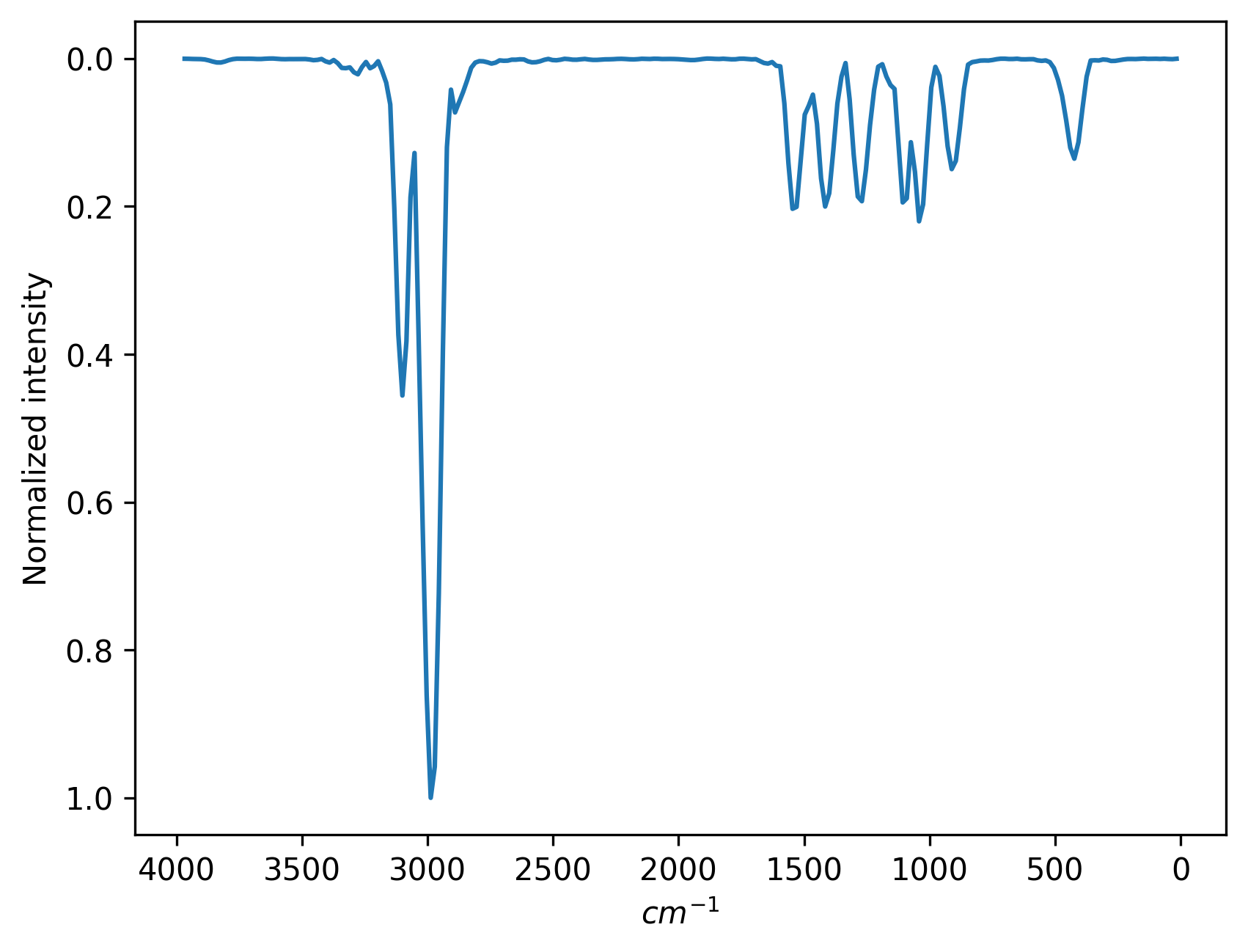
The keyword output is used to control which kind of vibrational spectrum to calculate. output=ir gives infrared spectrum and output=ps gives power spectrum. Below is the input file that calculates power spectrum.
MD2vibr # 1. requests vibrational spectra from MD trajectory
trajH5MDin=ethanol_traj.h5 # 2. file with MD trajectory in h5md format
dt=0.5 # 3. time step of trajectory; unit: fs
start_time=0 # 4. use trajectory starting from 0 fs
end_time=10000 # 5. use trajectory ending at 10000 fs
autocorrelationDepth=1024 # 6. autocorrelation depth; unit: fs
zeropadding=1024 # 7. zero padding length; unit: fs
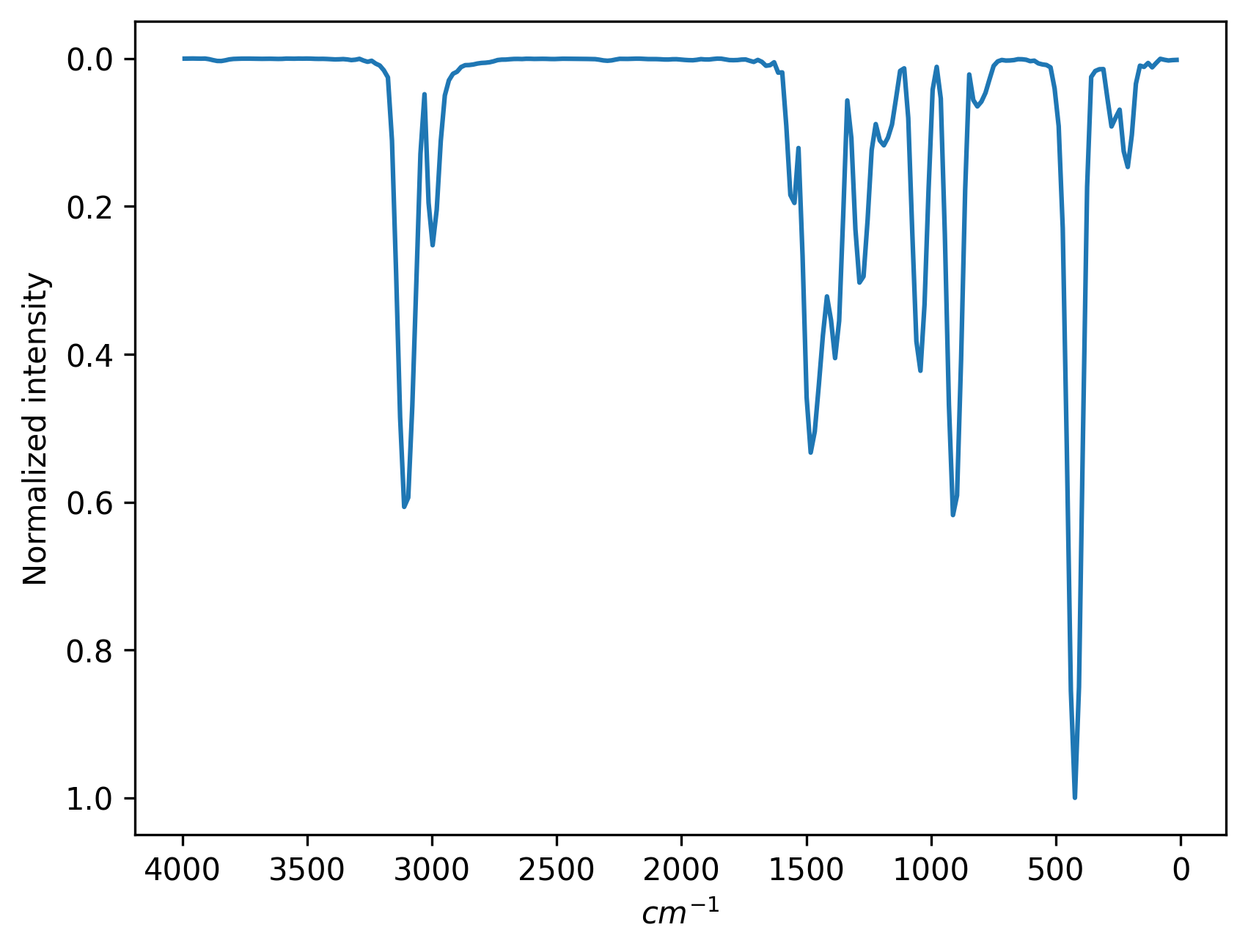
output=ps # 8. output power spectrum
The power spectrum should look like this:
Apart from MD trajectories in h5md format, users can also provide dipole moments (for infrared spectrum) or velocities (for power spectrum) in plain text, where keyword trajdpin or trajVXYZin is used. Below are examples of two cases.
MD2vibr                    # 1. requests vibrational spectra from MD trajectory
trajdpin=ethanol_traj.dp   # 2. file with dipole moments in plain text
dt=0.5                     # 3. time step of trajectory; unit: fs
start_time=0               # 4. use trajectory starting from 0 fs
end_time=10000             # 5. use trajectory ending at 10000 fs
autocorrelationDepth=1024  # 6. autocorrelation depth; unit: fs
zeropadding=1024           # 7. zero padding length; unit: fs
output=ir                  # 8. output infrared spectrum
MD2vibr                       # 1. requests vibrational spectra from MD trajectory
trajVXYZin=ethanol_traj.vxyz  # 2. file with velocities in plain text
dt=0.5                        # 3. time step of trajectory; unit: fs
start_time=0                  # 4. use trajectory starting from 0 fs
end_time=10000                # 5. use trajectory ending at 10000 fs
autocorrelationDepth=1024     # 6. autocorrelation depth; unit: fs
zeropadding=1024              # 7. zero padding length; unit: fs
output=ps                     # 8. output power spectrum
Note
In principle, our default recommendation is to use AIQM1 as it is usually the most accurate method for affordable cost. The dipole moments are extracted from the ODM2* part of AIQM1. However, they are only available when you use MNDO program as QM part. We recommend to install the MNDO to unlock the full potential of AIQM1. The XACS cloud uses Sparrow instead, which currently does not provide dipole moments and only provides numerical gradients limiting its applicability for MD. Another limitation is that AIQM1 is currently only applicable to the compounds with CHNO elements. ANI-1ccx is a good alternative on the XACS cloud if it can be applied but it does not provide dipole moments either (it has additional limitations to neutral closed-shell compounds in ground state).
Other keywords
Keywords start_time and end_time control which part of trajectory is used to calculate the spectrum. By default, MLatom will use the whole trajectory. autocorrelationDepth controls the autocorrelation depth which affects the peak widths while zeropadding controls how many zeros are appended to calculated autocorrelation function which affects the resolution of the spectrum. These two settings are by default 1024 fs. MLatom will normalize the spectrum by the maximum intensity. If you want the original spectrum, you can use the keyword normalize_intensity=0.
Using API
Below shows how to calculate vibrational spectra via MLatom API.
import mlatom as ml

# Loading MD trajectory in h5md format
traj = ml.data.molecular_trajectory()
traj.load(filename='ethanol_traj.h5',format='h5md')
moldb = ml.data.molecular_database()
moldb.molecules = [step.molecule for step in traj.steps]

# Loading MD trajectory in plain text
# moldb = ml.data.molecular_database.from_xyz_file('ethanol_traj.xyz')
# moldb.add_xyz_vectorial_properties_from_file('ethanol_traj.vxyz','xyz_velocities')
# with open('ethanol_traj.dp','r') as f:
#     lines = f.readlines()
# for ii in range(len(moldb)):
#     moldb[ii].dipole_moment = [float(each) for each in lines[ii].strip().split()]

# Calculate vibrational spectra
vibr = ml.vibrational_spectrum(molecular_database=moldb,dt=0.5)

# Infrared spectrum
freqs_ir,ints_ir = vibr.plot_infrared_spectrum(filename='ethanol_ir.png',  # file to save the figure
                                               autocorrelation_depth=1024, # autocorrelation depth; unit: fs
                                               zero_padding=1024,          # zero padding; unit: fs
                                               lb=0,                       # start time; unit: fs
                                               ub=10000,                   # end time; unit: fs
                                               normalize=True,             # normalize the spectrum
                                               return_spectrum=True,       # get the spectrum array from the function
                                               format='modulus')           # use the modulus of the dipole moments
# Power spectrum
freqs_ps,ints_ps = vibr.plot_power_spectrum(filename='ethanol_ps.png',     # file to save the figure
                                            autocorrelation_depth=1024,    # autocorrelation depth; unit: fs
                                            zero_padding=1024,             # zero padding; unit: fs
                                            lb=0,                          # start time; unit: fs
                                            ub=10000,                      # end time; unit: fs
                                            normalize=True,                # normalize the spectrum
                                            return_spectrum=True)          # use the modulus of the dipole moments

# Save the spectra
np.save('ethanol_ir_saved.npy',np.array((freqs_ir,ints_ir)))
np.save('ethanol_ps_saved.npy',np.array((freqs_ps,ints_ps)))
The keywords are slightly different from that in the input file. The user can use lb and ub to control the start time and end time of the trajectory. autocorrelation_depth and zero_padding can be used to tune the autocorrelation depth and zero padding. Normalization to the maximum intensity is enabled if normalize=True. The user can get frequencies and intensities from the return value of the function by using return_spectrum=True. In infrared specturm, the user can either use the modulus or XYZ vector of dipole moments by using format='modulus' or format='vector'.
Any questions or suggestions?
If you have further questions, criticism, and suggestions, we would be happy to receive them in English or Chinese via email, Slack (preferred), or QQ (135258964). See our contact page for more information on how to subscribe to updates and follow us on social media.