Transition states
In this tutorial we show how to optimize and check the nature of the transition state (TS) geometry with MLatom. We will use the Diels–Alder reaction between ethylene and 1,3-butadiene as an example.

We also created a video covering the contents of this tutorial. You can find this video on Youtube.
Since MLatom supports various methods including QM methods, pre-defined and user-defined ML methods and hybrid QM/ML methods as is shown in overview. Here we choose the fast and popular semi-empirical method GFN2-xTB and you can check below how to use, e.g., AIQM1 (general-purpose hybrid QM/ML method) and B3LYP/6-31G*, and pure ML models (pre-trained or trained by user).
TS geometry optimization
Optimizing TS geometry can be quite complicated (see below what you can do in such cases). However, if you have a good initial guess for its structure, it might work quite well. Here we provide a good initial guess as an example (in Angstrom):
16

C          0.48462430     -0.55755495      1.43729151
C          0.48462430     -0.55755495     -1.43729151
C         -0.27595797     -1.44977527      0.70359025
C         -0.27595797     -1.44977527     -0.70359025
C         -0.27595797      1.45086377      0.69299925
C         -0.27595797      1.45086377     -0.69299925
H          0.37292526     -0.50748993      2.51767690
H          1.44526264     -0.21636383      1.06867438
H          0.37292526     -0.50748993     -2.51767690
H          1.44526264     -0.21636383     -1.06867438
H         -1.05536225     -2.01444047      1.21328943
H         -1.05536225     -2.01444047     -1.21328943
H          0.51071931      1.96707995      1.23581344
H         -1.20625330      1.32768072      1.23591744
H          0.51071931      1.96707995     -1.23581344
H         -1.20625330      1.32768072     -1.23591744
If everything goes well, you would need an input which is not too different from the usual input for the geometry optimization of minima, you would just need to replace geomopt with TS in your input file (command-line option):
GFN2-xTB                # 1. define QM method or ML or QM/ML model
TS                      # 2. request TS geometry optimization
xyzfile=da_ts_init.xyz  # 3. initial geometry guess
optxyz=da_ts_opt.xyz    # 4. file with optimized geometry
In Python API, the code would also require a small modification by adding ts=True as an option for the optimization routine:
import mlatom as ml

# Get the initial guess for the molecules to optimize
initmol = ml.data.molecule.from_xyz_file('da_ts_init.xyz')
# initmol charge and multiplicity can be changed if required, e.g., by uncommenting the lines below:
#initmol.charge = 1 ; initmol.multiplicity = 2

# Choose one of the predifined (automatically recognized) methods
mymodel = ml.models.methods(method='GFN2-xTB')
# or QM method, e.g., B3LYP with Gaussian
#mymodel = ml.models.methods(method='B3LYP/6-31G*', program='Gaussian')
# or hybrid QM/ML method
#mymodel = ml.models.methods(method='AIQM1')
# or ML model, e.g., MACE:
#mymodel = ml.models.mace(model_file='mace.pt')

# Optimize the geometry with the choosen optimizer:
geomopt = ml.optimize_geometry(model=mymodel, initial_molecule=initmol, ts=True, program='ASE', maximum_number_of_steps=10000)

# Get the final geometry
final_mol = geomopt.optimized_molecule
# and its XYZ coordinates
final_mol.xyz_coordinates

# Check and save the final geometry
print('Optimized coordinates:')
print(final_mol.get_xyz_string())
final_mol.write_file_with_xyz_coordinates(filename='da_ts_opt.xyz')

# You can also check the optimization trajectory
print('Number of optimization steps:', len(geomopt.optimization_trajectory.steps))
# and access any geometry during optimization as
intermediate_step_geom = geomopt.optimization_trajectory.steps[2].molecule
print('Intermediate coordinates:')
print(intermediate_step_geom.get_xyz_string())
The snippet from the MLatom’s output file when used in command-line mode (with the Gaussian optimizer, see other options and pitfalls):
==============================================================================
Optimization of molecule 1
==============================================================================

Iteration         Energy (Hartree)
            1            -17.8096315123480
            2            -17.8106949632610
            3            -17.8116884258690
            4            -17.8120367568860
            5            -17.8122673179990
            6            -17.8122596563090
            7            -17.8122592324260

Final energy of molecule      1:         -17.8122592324260 Hartree


==============================================================================
The final optimized geometry (in da_ts_opt.xyz file obtained in either way) is:
16

C             0.4813024374103          -1.4349227612885           0.5137386536117
C             0.4859702737149           1.4344889056846           0.5129530071391
C             1.2680466082266          -0.7096089630187          -0.3161249847856
C             1.2698482503147           0.7063075171378          -0.3168590194909
C            -1.5743749532249          -0.6736952829099          -0.2267301172749
C            -1.5741402429035           0.6770058850694          -0.2253736447211
H             0.4107820982713          -2.5048539561628           0.4024004256024
H             0.1545008650554          -1.0465393829088           1.4604758694958
H             0.4182444345553           2.5045006285090           0.4008820574544
H             0.1575374270938           1.0474822961018           1.4596556145266
H             1.7590868456084          -1.2036512202944          -1.1442175065287
H             1.7624326531584           1.1982575357438          -1.1452660986280
H            -1.9999454494089          -1.2291294376367           0.5911010005786
H            -1.4029477841077          -1.2229351940318          -1.1358103575475
H            -1.9978808718237           1.2312093010793           0.5942018379777
H            -1.4017244596312           1.2282076255495          -1.1330462098024
Checking TS
Once you found some reasonably looking TS, you need to check whether it is a correct structure.
The simplest check is to perform frequency calculations for the optimized structure (see our previous tutorial on frequency calculations) and then analyze how the normal mode with imaginary frequency looks like.
MLatom will save the gaussian.log file after frequency calculation with which you can easily check with your favorite GUI like GaussView.
We show below the vibration movie generated by GaussView on the normal mode with negative frequency (calculated by GFN2-xTB on XACS cloud):
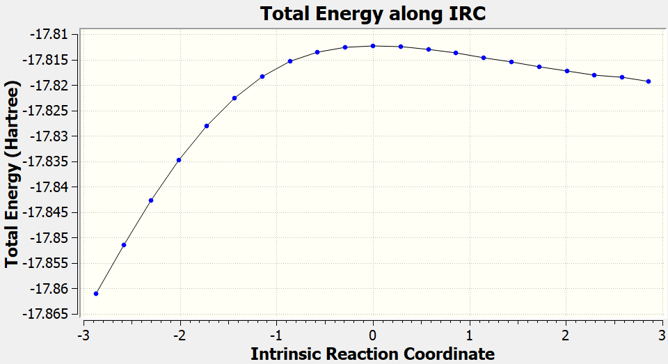
An additional standard check is performing intrinsic reaction coordinate (IRC) calculations (see details in this IRC tutorial), which are supported via Gaussian interface with input for MLatom as follows:
IRC
GFN2-xTB
xyzfile=da_ts_opt.xyz
In Python API, we will call mlatom.simulations.irc() to perform the IRC calculations.
You need to provide the model you use and the ts_molecule, i.e., the optimized TS geometry you want to check.
import mlatom as ml

# Get optimized molecules
optmol = ml.data.molecule.from_xyz_file('da_ts_opt.xyz')

# Choose one of the predifined (automatically recognized) methods
mymodel = ml.models.methods(method='GFN2-xTB')
# or QM method, e.g., B3LYP with Gaussian
#mymodel = ml.models.methods(method='B3LYP/6-31G*', program='Gaussian')
# or hybrid QM/ML method
#mymodel = ml.models.methods(method='AIQM1')
# or ML model, e.g., MACE:
#mymodel = ml.models.mace(model_file='mace.pt')

IRC = ml.simulations.irc(model=mymodel,ts_molecule=optmol)
After the IRC calculations finished, you can also check the gaussian.log file to plot the IRC curve (generated from geometry optimized by GFN2-xTB).
Dealing with complicated cases
Unfortunately, TS optimization does not always lead to the desired result. Hence, you might need to tinker more with the calculations settings and use, e.g., algorithms which take into account the geometries of reactant and product.
Currently, if you are familiar with the Gaussian program, our recommendation is to get gaussian.com input files from preliminary MLatom attempt at calculating TS and modify it accordingly by, e.g., using QST2 or QST3 methods.
Here is an example of such file for the Diels–Alder reaction:
%nproc=1
#p opt(qst3) external='/share/apps/anaconda3/bin/python3 /export/home/xacscloud/mlatom_versions/mlatom/interfaces/gaussian_interface.py'

reactants

0 1
C     0.484624300000     -0.557554950000      1.437291510000
C     0.484624300000     -0.557554950000     -1.437291510000
C    -0.275957970000     -1.449775270000      0.703590250000
C    -0.275957970000     -1.449775270000     -0.703590250000
C    -0.311976759298      2.284843109406      0.344043544386
C    -0.311976759298      2.284843109406     -1.041954955614
H     0.372925260000     -0.507489930000      2.517676900000
H     1.445262640000     -0.216363830000      1.068674380000
H     0.372925260000     -0.507489930000     -2.517676900000
H     1.445262640000     -0.216363830000     -1.068674380000
H    -1.055362250000     -2.014440470000      1.213289430000
H    -1.055362250000     -2.014440470000     -1.213289430000
H    -0.921357965784      1.567908780096      0.886857734386
H     0.545932937341      2.665125132700      0.886961734386
H    -0.921357965784      1.567908780096     -1.584769145614
H     0.545932937341      2.665125132700     -1.584873145614

products

0 1
C    -0.661894740000     -0.059709790000     -1.393910490000
C    -1.486209330000     -0.113548400000     -0.144719260000
C    -0.691627710000      0.317536480000      1.081726060000
C     0.691627710000     -0.317536480000      1.081726060000
C     1.486209330000      0.113548400000     -0.144719260000
C     0.661894740000      0.059709790000     -1.393910490000
H    -1.190276150000     -0.118797780000     -2.341761460000
H    -2.373254720000      0.518104980000     -0.263582030000
H    -1.871283790000     -1.133268850000     -0.007315520000
H    -1.235540190000      0.060874970000      1.994969250000
H    -0.583769070000      1.408342230000      1.074593440000
H     1.235540190000     -0.060874970000      1.994969250000
H     0.583769070000     -1.408342230000      1.074593440000
H     2.373254720000     -0.518104980000     -0.263582030000
H     1.871283790000      1.133268850000     -0.007315520000
H     1.190276150000      0.118797780000     -2.341761460000

TS

0 1
C     0.484624300000     -0.557554950000      1.437291510000
C     0.484624300000     -0.557554950000     -1.437291510000
C    -0.275957970000     -1.449775270000      0.703590250000
C    -0.275957970000     -1.449775270000     -0.703590250000
C    -0.275957970000      1.450863770000      0.692999250000
C    -0.275957970000      1.450863770000     -0.692999250000
H     0.372925260000     -0.507489930000      2.517676900000
H     1.445262640000     -0.216363830000      1.068674380000
H     0.372925260000     -0.507489930000     -2.517676900000
H     1.445262640000     -0.216363830000     -1.068674380000
H    -1.055362250000     -2.014440470000      1.213289430000
H    -1.055362250000     -2.014440470000     -1.213289430000
H     0.510719310000      1.967079950000      1.235813440000
H    -1.206253300000      1.327680720000      1.235917440000
H     0.510719310000      1.967079950000     -1.235813440000
H    -1.206253300000      1.327680720000     -1.235917440000
Note
Above input file is just for illustration as the path to your Python and MLatom installation should be different. You also need to run this file in the same folder (or its copy) where you perform the preliminary TS optimization as it generated additional required files such as model.json. Expert users can, of course, create their own model.json file.
Choosing the method or model
The user can benefit from MLatom’s many choices of the methods or models to be used for optimizations. You can check tutorial on single point calculation to get more details on how to define these types of methods. Here we give brief examples to quickly get started. There are many methods such as ANI-1ccx or AIQM1 which can be recognized automatically by MLatom as is illustrated in manual for API of models.
The general way to define the QM method is to use method and the corresponding QM program providing its implementations (MLatom uses interfaces to such programs). For example, ab initio (e.g., HF or MP2) or DFT (e.g., B3LYP/6-31G*) can be requested with the input:
method=B3LYPG/6-31G*    # 1. request running DFT optimization with B3LYP
qmprog=PySCF            # 2. request using PySCF for B3LYP calculations; qmprog=Gaussian can be also used
TS                      # 3. request transition state geometry optimization
xyzfile=da_ts_init.xyz  # 4. initial geometry guess
optxyz=da_ts_opt.xyz    # 5. file with optimized geometry
We provide here the comparison table for optimization time, iteration number, and RMSD with respect to the reference TS geometry (at B3LYP/6-31G*). All the calculations are performed on the XACS cloud.
method |
time (min) |
number of iterations |
RMSD (\(\unicode{x212B}\)) |
|---|---|---|---|
GFN2-xTB |
0.50 |
7 |
0.03 |
AIQM1 |
1.67 |
18 |
0.07 |
For this particular case, GFN2-xTB has excellent performance. However, AIQM1 is also quite good and, in fact, our larger scale benchmark showed that it is generally more robust and faster than GFN2-xTB. Hence, both methods can be recommended for pre-optimization of TS followed by DFT optimizations.
Note
AIQM1 is currently only applicable to the compounds with CHNO elements. Another limitation is that to unlock its full potential, we recommend to install the MNDO program for its QM part. The XACS cloud uses Sparrow instead, which currently only provides numerical gradients limiting its applicability for geometry optimizations.
The general way to request the optimization with the user-trained ML model is to specify the ML model type with MLmodelType and MLmodelIn keyword such as:
MLmodelType=MACE        # 1. request optimization with the MACE-type of machine learning potential
MLmodelIn=mace.pt       # 2. the file with the trained model should be provided, here it is mace.pt file
TS                      # 3. request transition state geometry optimization
xyzfile=init.xyz        # 4. initial geometry guess
optxyz=opt.xyz          # 5. file with optimized geometry
See manuals and tutorials on how to train such models, e.g., for MACE.
The advanced user-defined hybrid models such as those based on the delta-learning concept can be used for geometry optimizations only via Python API (see example in geometry optimization).
Choosing the optimization program
For transition state geometry optimization, MLatom supports the use of Gaussian and ASE optimizer. They can be chosen by adding optporg=[ASE, geometric or Gaussian] keyword as :
GFN2-xTB                # 1. define the method
TS                      # 2. requests transition state geometry optimization
xyzfile=init.xyz        # 3. initial geometry guess
optxyz=opt.xyz          # 4. file with optimized geometry
optprog=gaussian        # 5. Gaussian is choosen as the optimizer
If no optimizer is requested, MLatom will check the availability of the programs in the order Gaussian -> geometric -> ASE.
Each of the optimizers have their advantages and disadvantages:
ASE is open-source and tested by the community. It is available on the XACS cloud and can be easily installed.
GeomeTRIC is open-source and features its various choices for coordinate systems. Compared with Gaussian, it may take much more iterations to converge.
Gaussian is very versatile and time-tested program, allowing its users to exploit all Gaussian’s functionality as usual with additional benefit of access to ML models. It should be obtained and installed separately by the user. The I/O is currently not very efficient so that the optimizations with very fast ML models will take much longer than with other optimizers. It might be improved in the future.
Note
MLatom is being rapidly developed, so it will get more features and improved geometry optimization features. Our recommendations will change too. Please check from time-to-time this tutorial and also follow our updates on the usual channels.
Whatever optimizer you choose, it is worth checking the instructions below for pitfalls and tips.
ASE optimizer
Currently, TS optimization by ASE only supports dimer method. At some point, we are likely to implement nudge elastic band (NEB) too but it is not available yet.
Note
When dimer method is used, it always gives different result in the current MLatom implementation (it is default setting in ASE due to the use of the random seed). Hence, if you run the optimization several times, you will obtain different result each time (one of them can be what you are looking for). Compared to the Gaussian optimizer, dimer method can also take lots of iterations.
geomeTRIC optimizer
GeomeTRIC is an open-source software which introduce a new translation-rotation-internal coordinate (TRIC) system to describe molecule structure for efficient geometry optimization. It accepts external software for the energy and gradient, which is provided by various methods in MLatom, through wrapper functions. By default, geomeTRIC uses BFGS for optimization task.
On XACS cloud, geomeTRIC optimizer is the default option if optprog is not specified in input file and program is not set for mlatom.optimize_geometry() with python.
For example, you can try the input below using our newly updated UAIQM method to perform previous task on XACS cloud:
uaiqm                   # 1. define QM method or ML or QM/ML model
TS                      # 2. request TS geometry optimization
xyzfile=da_ts_init.xyz  # 3. initial geometry guess
optxyz=da_ts_opt_uaiqm.xyz    # 4. file with optimized geometry
And we provide the output file and optimized molecule as reference, as well as the results from frequency calcuclation as validation.
Gaussian optimizer
For the Gaussian optimizer, the calculation would be equal to using opt(ts,calcfc,noeigen,nomicro) in Gaussian input file (see gaussian.com file in your working directory).
When Gaussian optimizer is used, you will see the gaussian.log file which is similar to the common Gaussian output file with the difference, that it will use the MLatom’s model to predict energies and gradients to perform the geometry optimization.
Then you can use your favorite tools to analyze this output as usual for Gaussian, which is a big advantage for the Gaussian users.
The full Gaussian output file can be downloaded too.
An additional important advantage is that the advanced users can modify the gaussian.com file which contains the input required for transition state geometry optimization with MLatom’s models.
For example, as have illustrated in previous section, if you want to use various optimization algorithms in Gaussian, you can always modify the input file by replacing opt(ts) with opt(qst3) or other algorithms.
Also, in this way, the user can unlock the access to all the great Gaussian functionality for geometry optimizations such as freezing coordinates or defining input in internal coordinates, etc.
After the gaussian.com file is modified, you can run with it the Gaussian job as usual, e.g., in your system like g16 gaussian.com in the command line.
Any questions or suggestions?
If you have further questions, criticism, and suggestions, we would be happy to receive them in English or Chinese via email, Slack (preferred), or QQ (135258964). See our contact page for more information on how to subscribe to updates and follow us on social media.