Transfer learning
Transfer learning (TL) is an often-used technique in machine learning that helps you train better neural network models. The basic idea is to reuse the knowledge (parameters) of the pre-trained model from a different task, by fixing and changing some of its layers and then fit the model for a new task. There are serval reasons that we might utilize this technique:
Better training performance
The pre-trained models can give you a good starting point to kick off the training, which helps the convergence and might improve the accuracy of the final model.
Less data hungry
Training from a pre-trained model does not require data as much as training from scratch, since the pre-trained model already contains tons of information from its training data. This can be critical, especially when the accessibility to the data for the new task is limited.
Note that the advantages might not be able to be realized unless you choose your pre-trained model and train it properly. E.g. you definitely don’t want to use a totally unrelated model as the pre-trained model.
Here we show two tutorials:
Transfer learning from the universal models
The training data, initial geometry for frequency calculation and the reference harmonic frequencies at MP2/zvtz level can be found in TL_tutorial.zip
Tutorial on transfer learning from universal models
In this tutorial, we will improve the universal machine learning potential ANI-1ccx-gelu specifically on CH3NO2 molecule, which will be reflected in improved harmonic frequencies compared with experiment
import mlatom as ml
import numpy as np
import pandas as pd
import matplotlib.pyplot as plt
Overview of the dataset
We take the datasets from https://doi.org/10.1021/acs.jctc.1c00249. There are 9001 training points with energies and forces at MP2/aug-cc-pVTZ level.
# prepare the dataset
training_data = ml.data.molecular_database.load('CH3NO2_MP2_avtz.json',format='json')
print('Number of training points: ', len(training_data))
Number of training points: 9001
# plot the energy distribution
energies = training_data.get_properties('energy')
plt.hist(energies)
plt.xlabel('Energy (Hartree)')
plt.ylabel('Number of entries')
Text(0, 0.5, 'Number of entries')

Load universal model
ani1ccx_gelu = ml.models.methods(method='ANI-1ccx-gelu')
# ani = ml.models.methods(method='ANI-1ccx')
# ani = ml.models.methods(method='ANI-2x')
If you just want to do transfer learning on one of the universal models, you can use model_index to load specific model.
ani1ccx_gelu_cv0 = ml.models.methods(method='ANI-1ccx-gelu', model_index=0)
Fine tune
There are several parameters we need to care about when transfer learning (though we have default settings in MLatom, you might want to customize the procedure yourself)
Arguments to pass to train()
The arguments available can be found in manual for API about torchani interface. Here several key arguments are listed:
reset_energy_shifter [list, bool]: Control how the self atomic energies will be extracted. By default we will use those extracted from the training data. If set to False, we will use those from pretrained models. If list, values inside will be used as the self atomic energies for scaling.file_to_save_model [str]: The file name to save the retrained models. Defaul "{universal model name}_retrained.pt.cv{model index}"verbose [bool or int]: Control the information printed out when training. 1 will print out training procedure and 2 will print out metrics from training and validation.hyperparameters [dict]: Control the training procedure, will explain in detail later.
Parameters in hyperparameters
batch_size: default 8max_epochs: default 100 for transfer learningfixed_layers: default 1 and 3 layer are fixed.
ani1ccx_gelu_cv0.train(
    molecular_database=training_data,
    property_to_learn='energy',
    xyz_derivative_property_to_learn = 'energy_gradients',
    verbose=0,
    hyperparameters={
        'batch_size':512,
        }
)
Start retraining on model 0...
After transfer learning, the ani1ccx_gelu_cv0 has been replaced by the new model and can be directly used for simulation. We also saved the model file in the current directory either named in the combination of the universal model name plus 'retrained' or the user defined name for the model. You can still load them with torchani interface to do the simulations:
# for loading one model
ani1ccx_gelu_cv0_retrained = ml.models.ani(model_file='ani1ccxgelu_retrained.pt.cv0')
model loaded from ani1ccxgelu_retrained.pt.cv0
Compare harmonic frequencies
def calculate_harmonic_frequency(
    calculator=None,
    initmol=None,
    opt_program='geometric', # do not use gaussian which currently cannot recognize the retrained method
    freq_program='pyscf',

):
    geomopt = ml.simulations.optimize_geometry(
        model=calculator,
        initial_molecule=initmol,
        program=opt_program)
    optmol = geomopt.optimized_molecule
    ml.simulations.freq(
        model=calculator,
        molecule=optmol,
        program=freq_program,)
    return optmol
# load initial molecule
initmol = ml.data.molecule.from_xyz_file('CH3NO2_init.xyz')

# load universal model
ani1ccx_gelu_original_cv0 = ml.models.methods(method='ANI-1ccx-gelu', model_index=0)
# calculate harmonic frequency
freqmol_anigelu_original = calculate_harmonic_frequency(ani1ccx_gelu_original_cv0, initmol)
freqmol_anigelu_cv0 = calculate_harmonic_frequency(ani1ccx_gelu_cv0, initmol)
# load performance table and check MAE
reference_table = pd.read_csv('CH3NO2_harmonic.csv')
reference_table['ANI-1ccx-gelu-cv0'] = freqmol_anigelu_original.frequencies
reference_table['ANI-1ccx-gelu-cv0-TL'] = freqmol_anigelu_cv0.frequencies

print('MAE (cm-1) of harmonic frequencies compared to MP2:')
mae = abs(reference_table['ANI-1ccx-gelu-cv0'].astype(np.float32)-reference_table['MP2/avtz'].astype(np.float32)).mean()
print(f'ANI-1ccx-gelu-cv0: {mae}')
mae = abs(reference_table['ANI-1ccx-gelu-cv0-TL'].astype(np.float32)-reference_table['MP2/avtz'].astype(np.float32)).mean()
print(f'ANI-1ccx-gelu-cv0-TL: {mae}')
MAE (cm-1) of harmonic frequencies compared to MP2:
ANI-1ccx-gelu-cv0: 26.988115310668945
ANI-1ccx-gelu-cv0-TL: 7.507749557495117
reference_table
| Model | MP2/avtz | exp | ANI-1ccx-gelu-cv0 | ANI-1ccx-gelu-cv0-TL | |
|---|---|---|---|---|---|
| 0 | 1 | 28.91 | - | 103.767999 | 64.703797 |
| 1 | 2 | 478.65 | 479 | 513.901562 | 479.278102 |
| 2 | 3 | 610.43 | 599 | 622.286085 | 616.218573 |
| 3 | 4 | 669.67 | 647 | 672.347919 | 672.521882 |
| 4 | 5 | 940.48 | 921 | 965.608931 | 943.043952 |
| 5 | 6 | 1127.28 | 1097 | 1118.818235 | 1125.426629 |
| 6 | 7 | 1148.99 | 1153 | 1120.208904 | 1143.753734 |
| 7 | 8 | 1412.12 | 1384 | 1417.408563 | 1406.389784 |
| 8 | 9 | 1430.54 | 1413 | 1462.599118 | 1418.542115 |
| 9 | 10 | 1491.90 | 1449 | 1477.057543 | 1481.028898 |
| 10 | 11 | 1502.67 | 1488 | 1481.334926 | 1504.267194 |
| 11 | 12 | 1745.72 | 1582 | 1649.090329 | 1757.063420 |
| 12 | 13 | 3115.24 | 2965 | 3096.578013 | 3123.332056 |
| 13 | 14 | 3221.29 | 3048 | 3215.941830 | 3214.247684 |
| 14 | 15 | 3247.61 | 3048 | 3223.968831 | 3248.836237 |
Note
Fine-tuning for the universal models is supported for ANI-type models ANI-1x, ANI-1ccx, ANI-1ccx-gelu, and ANI-2x.
When using this feature, please cite:
Seyedeh Fatemeh Alavi, Yuxinxin Chen, Yi-Fan Hou, Fuchun Ge, Peikun Zheng, Pavlo O. Dral*. ANI-1ccx-gelu Universal Interatomic Potential and Its Fine-Tuning: Toward Accurate and Efficient Anharmonic Vibrational Frequencies. J. Phys. Chem. Lett. 2025, 16, 483–493. DOI: https://doi.org/10.1021/acs.jpclett.4c03031.
Preprint on ChemRxiv: https://doi.org/10.26434/chemrxiv-2024-c8s16 (2024-10-09).
Transfer learning from scratch
A typical transfer learning scheme includes:
Obtain the pre-trained model
Fix/change layers
Retrain
The first and last steps can be easily done in the normal MLatom routine (via model.__init__(model_file) and model.train()). While the second one might be a little bit complicated: we need to modify model.model.
Although platforms like PyTorch, Tensorflow have the flexibility to allow users to modify the model as they wish. This modification still requires a little bit deeper knowledge about the model’s architecture.
Fortunately, we provide some shortcut methods in our interface to TorchANI, to make it easier to fix some of the layers in a model (no quick methods for adding layers / other interfaces yet…).
Let’s see how it works.
ANI TL model
Here we just use hydrogen molecule as a simple example. The Jupyter notebook can be downloaded from the bottom of this page.
First we need to generate some data.
import mlatom as ml
import numpy as np
import matplotlib.pyplot as plt

# prepare H2 geometries with bond lengths ranging from 0.5 to 5.0 Å
xyz = np.zeros((451, 2, 3))
xyz[:, 1, 2] = np.arange(0.5, 5.01, 0.01)
z = np.ones((451, 2)).astype(int)
molDB = ml.molecular_database.from_numpy(coordinates=xyz, species=z)

# calculate HF energies
hf = ml.models.methods(method='HF/STO-3G', program='PySCF')
hf.predict(molecular_database=molDB, calculate_energy=True)
molDB.add_scalar_properties(molDB.get_properties('energy'), 'HF_energy') # save HF energy with a new name

# calculate CISD energies
cisd = ml.models.methods(method='CISD/cc-pVDZ', program='PySCF')
cisd.predict(molecular_database=molDB, calculate_energy=True)
molDB.add_scalar_properties(molDB.get_properties('energy'), 'CISD_energy')
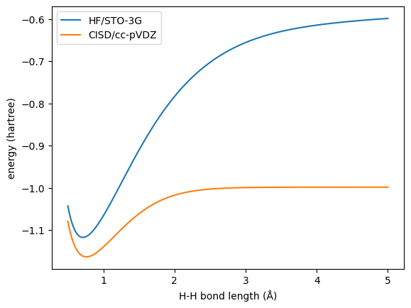
Here we use HF/STO-3G and CISD/cc-pVDZ to generate two levels of energies for the geometry whose H-H bond lengths ranging from 0.5 to 5.0 Å.
Then we can train an ANI model with HF energies to be the pre-trained model.
# train ANI model with HF energies
ani = ml.models.ani(model_file='ANI-HF.pt', verbose=False)
ani.train(molecular_database=molDB, property_to_learn='HF_energy')
# predict with trained ANI model
ani.predict(molecular_database=molDB, property_to_predict='ANI_HF_energy')
The model has a default structure as below:
Sequential(
(0): AEVComputer()
(1): ANIModel(
    (H): Sequential(
    (0): Linear(in_features=48, out_features=160, bias=True)
    (1): CELU(alpha=0.1)
    (2): Linear(in_features=160, out_features=128, bias=True)
    (3): CELU(alpha=0.1)
    (4): Linear(in_features=128, out_features=96, bias=True)
    (5): CELU(alpha=0.1)
    (6): Linear(in_features=96, out_features=1, bias=True)
    )
  )
)
Now let’s do transfer learning.
For this, you need to copy the file ANI-HF.pt with the model pre-trained on HF to ANI-HF-TL.pt file which will be used for fine-tuning on CISD.
# let's copy the model file to a new one, because it will be overwritten
! cp ANI-HF.pt ANI-HF-TL.pt

# fix some of the layers
ani = ml.models.ani(model_file='ANI-HF-TL.pt', verbose=False)
ani.fix_layers([[0, 6]])
# transfer leaning with every 40th of the data
step = 40
val = molDB[::step][::10]
sub = ml.molecular_database([mol for mol in molDB[::step] if mol not in val])
ani.energy_shifter.self_energies = None # let the model recalculate the self atomic energies
ani.train(molecular_database=sub, validation_molecular_database=val, property_to_learn='CISD_energy', hyperparameters={'learning_rate': 0.0001}, reset_optimizer=True)
# predict with TL model
ani.predict(molecular_database=molDB, property_to_predict='ANI_TL_energy')
Here, we only use 12 CISD data points (subtrain/validate: 10/2) to train the TL model.
And we fixed the first and the last linear layer in the model with ani.fix_layers([[0, 6]]) (see mlatom.interfaces.torchani_interface.ani.fix_layers).
Also, we change the initial learning rate to a smaller value to make the training less aggressive.
Next, let’s train another model with the same data from scratch.
# train ANI model with CISD energies directly
ani_cisd = ml.models.ani(model_file='ANI_CISD.pt', verbose=False)
ani_cisd.train(molecular_database=sub, validation_molecular_database=val, property_to_learn='CISD_energy')
# predict with trained ANI model
ani_cisd.predict(molecular_database=molDB, property_to_predict='ANI_CISD_energy')
Now let’s check the results.
# plot the energies
plt.plot(xyz[:, 1, 2], molDB.get_properties('HF_energy'), label='HF/STO-3G')
plt.plot(xyz[:, 1, 2], molDB.get_properties('CISD_energy'), label='CISD/cc-pVDZ')
plt.plot(xyz[:, 1, 2], molDB.get_properties('ANI_HF_energy'), label='ANI-HF')
plt.plot(xyz[:, 1, 2], molDB.get_properties('ANI_TL_energy'), label='ANI-TL')
plt.plot(xyz[:, 1, 2], molDB.get_properties('ANI_CISD_energy'), label='ANI-CISD')
plt.plot(sub.xyz_coordinates[:, 1, 2], sub.get_properties('CISD_energy'), 'o', label='TL subtraining')
plt.plot(val.xyz_coordinates[:, 1, 2], val.get_properties('CISD_energy'), 'o', label='TL validation')
plt.legend()
plt.xlabel('H-H bond length (Å)')
plt.ylabel('energy (hartree)')
plt.show()
First, we can see that the ANI-HF model trained with all the data has excellent agreement with the reference.
While for the CISD level, the transfer learned model behave way better than the direct one.
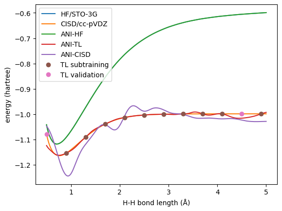
With this example, we can see the power of transfer learning: lower-level pre-trained model can boost the higher-level model even with a small training set.