1. Machine learning basics
1.1. Slides
1.2. Power of ML
Power of ML that it can make fast and accurate.
For example, let’s use the pure ML model trained for the hydrogen molecule to optimize its geometry:
Example ML-basics-1.
Calculate the bond length in H2 molecule with machine learning (ML) (see instructions below).
Write down:
Bond length you obtained.
How much time it took to complete the calculations.
The MLatom@XACS input file (h2_opt_kreg.inp) is pretty self-explanatory:
geomopt                # Request geometry optimization
MLmodelType=KREG       # with the ML model of the KREG type
MLmodelIn=energies.unf # in energies.unf file
XYZfile='
2

H             0.000           0.000           0.000
H             0.000           0.000           0.800
'
optXYZ=eq_KREG.xyz     # optimized geometry output
You also need to upload the file with ML model energies.unf as auxiliary file on the XACS cloud.
After you clicked the Submit button, you should have gotten the result pretty fast. On my computer, it took only ~0.3 seconds to obtain the bond length of 0.7415 Å. This is remarkably close to both experiment and FCI/aug-cc-pV6Z, but obtained much faster!
You can see for yourself that such calculations even for the hydrogen molecule are quite slow with FCI/aug-cc-pV6Z while with other methods like DFT you might not get very accurate result and it will still be slower.
Now you see, why computational chemists are so excited about using ML as it breaks through the limitations of slow QM methods and delivers results fast. It can be as accurate as we need if we train it on enough data. It can even achieve full CI accuracy in less than a second. Indeed, this is what our ML model delivers – full CI quality result for the hydrogen molecule!
1.3. Training your first ML model
Our first examples with geometry optimizations were easy as you did not need to do any training of ML models. We will show in the next example how to train this model.
You can now proceed to train your own KREG model and use it to calculate the bond length:
Example ML-basics-2.
Train the ML model for the H2 molecule (see instructions below) and obtain the bond length with this model.
Write down:
How much time did it take to train the model?
What are the training and validation errors?
What is the bond length of H2 obtained with your model?
The MLatom@XACS input file (h2_train_KREG.inp) with expanation in comments:
createMLmodel           # Specify the task for MLatom
MLmodelType=KREG        # Specify the model type
MLmodelOut=energies.unf # Save model in energies.unf
XYZfile=h2.xyz          # File with XYZ geometries
Yfile=E_FCI_451.dat     # The file with FCI energies (in Hartree)
sigma=opt               # Optimize hyperparameter sigma
lgSigmaL=-4             # Lower bound of log2(sigma)
lambda=opt              # Optimize hyperparameter lambda
For now, do not worry about hyperparameters in input file, I will explain them in another lecture.
You need two auxiliary files with data:
E_FCI_451.dat- energies in Hartree.h2.xyz- geometries.
You can examine the data files to get an idea what they contain.
At the end of calculation, you can find in the output file that the training and validation errors (in Hartree) are very tiny showing that the model learned well the data. Also, you got with this model the same bond length of 0.7415 Å as with FCI/aug-cc-pV6Z.
We will discuss in the separate topic different types of ML potentials and how to train, evaluate, and use them.
1.4. ML algorithms
The topic of ML algorithms is vast and I definetely can’t cover it fully as a part of a short lecture. Here I just provide very cursary discussion about the crucial points.
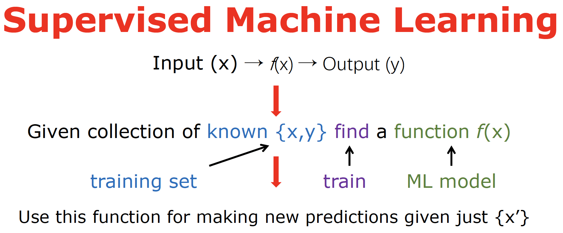
First of all, there are tons of different types of ML, including supervised, unsupervised, semi-supervised, self-supervised, and reinforcement learning. Here I only cover the most widely used supervised learning. The idea behind the supervised learning is summarized in this scheme:

Basically, we want to find an approximating function f (called ML model) that for a new input vector x’ would output y’ as close as possible to the true answer. We need to find this approximating function (the process called training) from the known set of data {x, y} called the training set. The goal of ML is not to fit the existing data as good as possible – we can just memorize them! The goal is to generalize to new, unseen points as good as possible.
What do we need for finding such a function?
data
choice of x (also called features or descriptor)
choice of y (reference values, labels)
fitting function (ML algorithm, ML model type)
optimize ML model parameters
There are tons of ML algorithms. The list is long and you can read up on them elsewhere:
various types of neural networks (NN), deep learning
kernel methods
Gaussian processes (GP)
kernel ridge regression (KRR)
support vector machines (SVMs) & support vector regression (SVR)
linear regression!
decision trees, random forest
k-nearest neighbor
and many more…
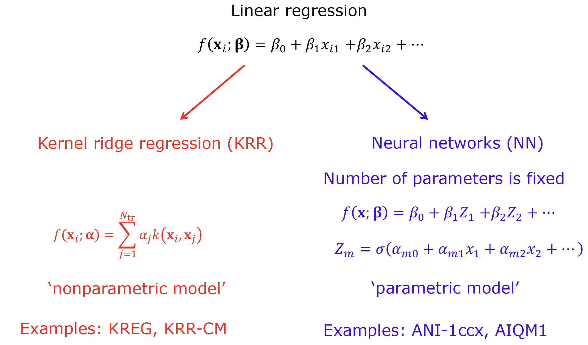
In my view, even linear regression satisfies the definition of a supervised ML model although some experts disagree. While linear regression is the simplest, it can be viewed as a starting point for more complex kernel methods (e.g., KRR) and NNs:

You have already used several ML types: KREG which is based on the KRR algorithm as well as UAIQM models which use NNs. The crucial difference between KRR and NNs is that the approximating function in KRR includes the training points explicitly in its functional expression (hence, it is sometimes referred to as memory-based) and, hence, the function expression depends on the training points. In contrast, algorithms like linear regression and NN, assume the fixed functional form. Both KRR and NN are capable of treating nonlinear problems but via different mechanisms. In KRR the input vector x is mapped into a higher-dimensional input space via the so called kernel function k(x, x’) which is often nonlinear (e.g., the Gaussian function). In NN, the linear output is transformed via a nonlinear activation function; the outputs can be fed into another such function giving rise to layers and deep networks have many layers (the input and output elements of the layers are called neurons or units).
The key practical difference is that for KRR we have an analytical solution to finding its parameters (regression coefficients) while for NN we do not and have to optimize its parameters (called weights and biad weights) iteratively in many iterations (called epochs) through the back-propagation (updating parameters based on how they impact the error called loss with different learning rate). The good news is that the back-propagation is well-parallelizable so that the processed data can be split in batches and calculations can be performed on GPUs which are more efficient (but more expensive!) than using CPUs.
The problem with NNs is that we end up with different networks even if train on the same data, because NNs do not have analytical solution and their initial weights are initialized randomly. This is bad and good news at the same time. The bad news is that NN optimization is not deterministic but the good news is that we can exploit it. For example, if we train multiple models, we can bundle them in an ensemble, average their predictions to obtain more stable result, and use the deviation between predictions of NNs as the metric for uncertainty as we have already seen for ANI-1ccx and AIQM1 which use eight networks.
Several additional important comments concerning the MLPs. Input matters too. Although we do provide XYZ coordinates as initial input, they are transformed in other more suitable descriptors, e.g., in KREG – into inverse internuclear distances, in UAIQM – so called local descriptors. Some NNs are able to iteratively update the descriptor (e.g., MACE and PhysNet – machine learning potentials covered separately) which are slower but promises ot deliver more accurate result. Also, some networks like MACE make use of equivariant input which is reacher on information and also provides better results (but slower).