4. Spectroscopy
Spectroscopy simulations are very important for bridging the theoretical understanding of molecular structure and reactivity with the experimental measurements. QM spectroscopy is typically quite expensive and here ML can help both as a surrogate, faster replacement of QM methods or be used to directly predict spectra. Also, there is long-standing interest in using ML for interpreting spectra and, most importantly, to obtain structures from spectra, but this is much more difficult and less mature. Here we can’t cover all types of spectroscopy but show on several common types how they can be simulated and what we should pay attention to when setting up the simulations.
4.1. Slides
4.2. (Ro)vibrational spectra
Rotational-vibrational (rovibrational), i.e., infrared (IR) and Raman, spectroscopy provides a direct way to probe the molecular structure. Hence, such spectra simulations have big practical importance. Their accurate simulations with QM methods are, however, rather expensive. ML is used to significantly accelerate such simulations.
Plenty of approaches were suggested for rovibrational spectra simulations of molecules. Most of them require the PES representation of a molecule which allow to calculate vibrational frequencies. However, calculations of intensities also require the knowldge of dipole moments and, often, their first- and second-order derivatives which are not always available (particularly with many ML methods). Two big classes considered here are the static and dynamic approaches. The static calculations are faster but miss the effects of the different distribution of conformers and often, also, can’t adequately describe the anharmonic effects. Dynamic approaches, on the other hand, often, inadequatly describe quantum nuclear effects.
4.2.1. IR from frequency calculations
Vibrational spectra can be calculated statically by just performing single-point calculations which require the costly evaluation of the Hessian matrix (second-order energy derivatives). The Hessian is diagonalized to obtaine frequencies and normal modes of vibrations. As you know, these properties are obtained by simply performing the frequency calculations using the freq keyword in MLatom. However, if you analyze the output file, you will discover that no intensities are predicted. Indeed, frequency calculations are just part of the answer, you need to know intensities to actually obtain the IR spectrum which can be compared to experiment.
Calculation of IR intensities, however, requires the evaluation of the first-order dipole moment derivatives with respect to normal mode coordinates. This is much more expensive and also not available in all models. To request such calculations, you can use the ir keyword in MLatom:
Simulating infrared spectra with UAIQM methods using input file in MLatom is ultra easy with only 3 lines.
Example ML-spectra-1.
Calculate IR spectrum of ethanol molecule with MLatom using static approach.
Analyze output file. How many normal modes does the molecule have?
Does the spectrum agrees well with experiment?
ir
uaiqm_wb97x631gp@cc
xyzfile=opt.xyz
where the opt.xyz is the ethanol optimized by uaiqm_wb97x631gp@cc as:
9

C             1.2141461144075          -0.2237522351565           0.0000009660331
H             1.2725810451795          -0.8571489137580          -0.8839209229985
H             1.2725955610560          -0.8571196861893           0.8839423252131
H             2.0641316742868           0.4586264688194          -0.0000176008701
C            -0.0820255073362           0.5506969112630          -0.0000006009490
H            -0.1394716683438           1.1910011723471           0.8856982674255
H            -0.1394676608187           1.1909953759585          -0.8857037188954
O            -1.1431943032587          -0.3953014469416          -0.0000014007109
H            -1.9775381677168           0.0743891017157           0.0000106653069
Warning
Always remember to optimize your molecule at the same level!
Vibrational analysis and IR intensities can be found in MLatom output files:
==============================================================================
                  Vibration analysis for molecule      1
==============================================================================
Multiplicity: 1
This is a nonlinear molecule
Mode     Frequencies     Reduced masses     Force Constants       IR intensities
            (cm^-1)            (AMU)           (mDyne/A)              (km/mol)
    1        241.0374          1.1507             0.0394                86.1148
    2        297.4762          1.0709             0.0558                54.1970
    3        418.2334          2.5803             0.2659                12.4199
    4        810.5925          1.0759             0.4165                 0.0530
    5        910.3415          2.1135             1.0319                12.0631
    6       1048.6773          1.8779             1.2167                48.5102
    7       1125.4218          2.7007             2.0154                37.0761
    8       1193.0919          1.5109             1.2672                 5.4162
    9       1274.9990          1.2567             1.2037                83.6804
    10       1305.5061          1.1150             1.1196                 0.0292
    11       1404.9278          1.2383             1.4401                 2.1079
    12       1454.1580          1.4707             1.8323                16.1926
    13       1493.5120          1.0405             1.3674                 5.3892
    14       1508.6873          1.0534             1.4126                 3.9672
    15       1539.9937          1.0936             1.5280                 2.0331
    16       2996.6657          1.0554             5.5840                65.1341
    17       3032.2203          1.1085             6.0050                66.4608
    18       3037.2688          1.0350             5.6253                14.7477
    19       3120.1171          1.1012             6.3160                27.1681
    20       3126.3285          1.1032             6.3532                28.7563
    21       3844.2694          1.0659             9.2813                22.8496
==============================================================================
                    Thermochemistry for molecule      1
==============================================================================
Selected UAIQM method: uaiqm_wb97x631gp@cc
Selected version: latest

Standard deviation of ML contribution    :      0.00014563 Hartree         0.09139 kcal/mol
Baseline contribution                    :   -154.98764057 Hartree
NN contribution                          :      0.09856558 Hartree
D4 contribution                          :     -0.00044829 Hartree
Total energy                             :   -154.88952328 Hartree

ZPE-exclusive internal energy at      0 K:      -154.88952 Hartree
Zero-point vibrational energy            :         0.08015 Hartree
Internal energy                  at   0 K:      -154.80937 Hartree
Enthalpy                         at 298 K:      -154.80413 Hartree
Gibbs free energy                at 298 K:      -154.83475 Hartree

Atomization enthalpy             at   0 K:         1.25151 Hartree       785.33412 kcal/mol
ZPE-exclusive atomization energy at   0 K:         1.33166 Hartree       835.63152 kcal/mol
Heat of formation                at 298 K:        -0.12976 Hartree       -81.42550 kcal/mol

==============================================================================
Here is the IR spectrum obtained with UAIQM:
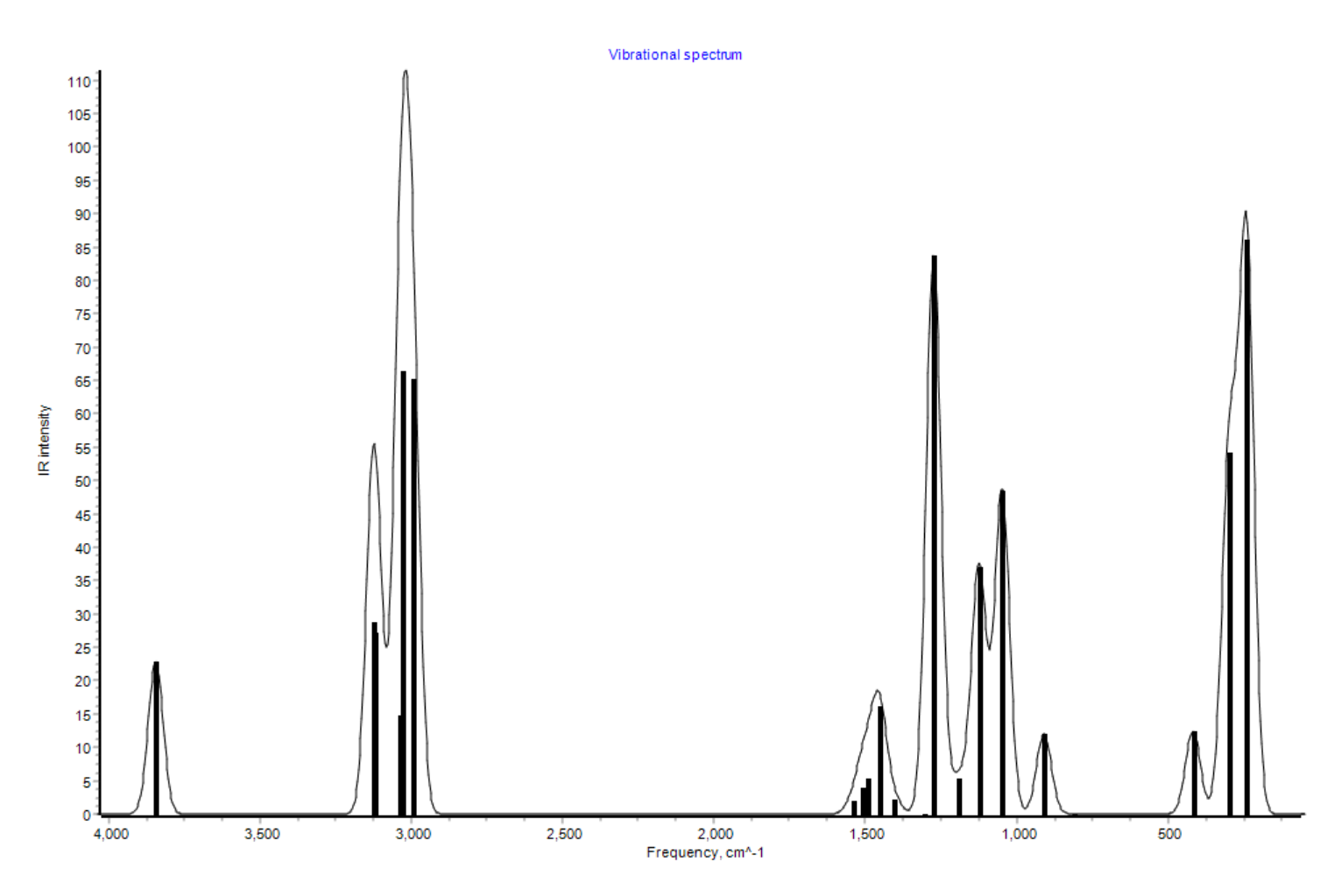
It is in quite a good agreement with the experimental spectrum available on NIST (you should compare to the gas phase IR spectrum as calculations are done in vacuum!).
Note
Currently, IR intensities can only be obtained with DFT-based UAIQM methods, i.e. uaiqm_wb97x631gp@cc, and uaiqm_wb97xdef2tzvpp@cc. Pure DFT methods are also supported. AIQM1 only locally supported.
4.2.2. IR and power spectra from MD
Rovibrational spectra can be obtained by simulating the nuclear motion with MD. The advantage is that this way the anharmonic effects are naturally included as well as conformational landscape can be properly represented. The disadvantage is that very long trajectories are needed which are quite expensive to obtain with the non-ML approaches. Also, classical MD does not properly take into account quantum nuclear effects which are especially substantial for light element hydrogen.
Similarly to frequency calculations, if we do not have dipole moments, we can only calculate the power spectra using the autocorrelation function of velocities in the MD trajectory. If dipole moments are available, you can calculate the IR spectra with intensities derived the fast Fourier transform of the autocorrelation function of dipole moments. That may sound complicated, but practically, MLatom provides the means to obtain both power and IR spectra by post-processing the MD trajectory (see a dedicated tutorial for more theory and calculation options). In the task below, you can calculate the IR spectrum from the trajectory and compare it to the spectrum from static calculations.
Example ML-spectra-2.
Calculate IR spectrum of ethanol molecule with MLatom from an MD trajectory which was calculated at AIQM1 level for 10 ps with 0.5 time step.
How does the spectrum compares to the spectrum from static calculations?
Compared to experiment, what are the major qualitative differences?
Input file:
MD2vibr                     # 1. requests vibrational spectra from MD trajectory
trajH5MDin=ethanol_traj.h5  # 2. file with MD trajectory in h5md format
dt=0.5                      # 3. time step of trajectory; unit: fs
start_time=0                # 4. use trajectory starting from 0 fs
end_time=10000              # 5. use trajectory ending at 10000 fs
autocorrelationDepth=1024   # 6. autocorrelation depth; unit: fs
zeropadding=1024            # 7. zero padding length; unit: fs
output=ir                   # 8. output infrared spectrum
Auxiliary files:
ethanol_traj.h5- trajectory in the h5md format, required for calculations.ethanol_traj.xyz- if you want to check how the trajectory looks like (not necessary for calculations)
After calculations finish, you will find ir.png with the plot of the infrared spectrum.
The major qualitative difference is that the high-frequency peaks are shifted despite an excellent accuracy of AIQM1: this is a known consequence of not including quantum nuclear effects. The future versions of MLatom will include path-integral MD to take into account these effects.
4.3. UV/vis absorption spectra
UV/vis absorption spectra is one of the most important spectroscopies which is also easy to carry out experimentally. However, theoretical simulations are very difficult because they require the calculation of excited states which are very costly and usually the affordable methods are not that accurate. There is therefore big insentive to accelerate and improve accuracy of theoretical UV/vis absorption spectra simulations with ML.
4.3.1. UV/vis spectra from single-point calculations
The simplest way to calculate UV/vis spectra is by optimizing the geometry in the ground state and calculating the excitation energies and oscillator strengths for this geometry. The oscillator strengths correspond to intensities via a simple relation and the common practice is to simply broaden the line spectra represented by excitation energies on the x-axis and oscillator strengths on the y-axis with a Gaussian function. The width of the Gaussian function is usually selected manually to match the experimental shapes. The peaks are sometimes shifted too. This is so-called single-point convolution approach and is commonly employed to obtain at least qualitative comparison with experiment and explain the origin of the absorption bands. We are planning to provide a simple input file implementation for this type of calculations in the near future.
4.3.2. UV/vis spectra with nuclear-ensemble approach
The problem with the single-point convolution is, as you might properly guess, that the molecules are not stationary objects and the excitation properties change as the molecule vibrates. An example is a benzene molecule which is highly symmetric in the ground-state minimum but the vibrations break the symmetry and some of the dark excitations become slightly observable as very weak peaks in UV/vis.
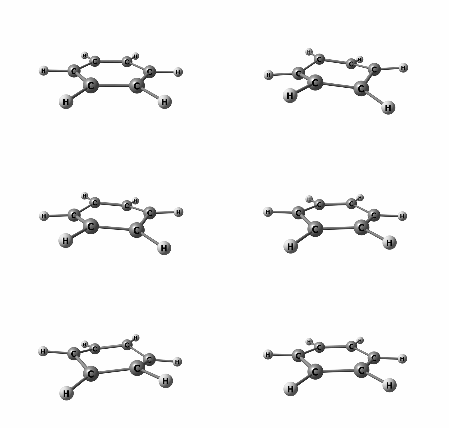
How to simulate such a process? We can sample many geometries from such vibrations – this collection of geometries is called nuclear ensemble. The geometries can be sampled from both MD and from the normal modes obtained with frequencies calculations (usually from the so-called Wigner distribution). The latter sampling is the easiest and most frequently employed. Once we have sampled the geometries, we can calculate the excitation properties for them and obtain a spectrum. Regardless how the ensemble is obtained, this method of calculating spectra is called nuclear ensemble approach (NEA). It is a more rigorous way of simulating UV/vis spectra as it can recover the absorption band shapes and positions better than single-point convolution.
However, NEA typically requires many hundreds or thousands of expensive quantum mechanical calculations of excited states precluding its widespread adoption. ML can greatly accelerate the simulations by predicting the excited state properties after learning on the fraction of the usually-required geometries. In our ML-NEA approach implemented in MLatom, we exploited the essence of ML – we can use the same program to learn different properties just given the data. This is in contrast to QM methods where we have first to derive the proper physical models and then implement them for each property:
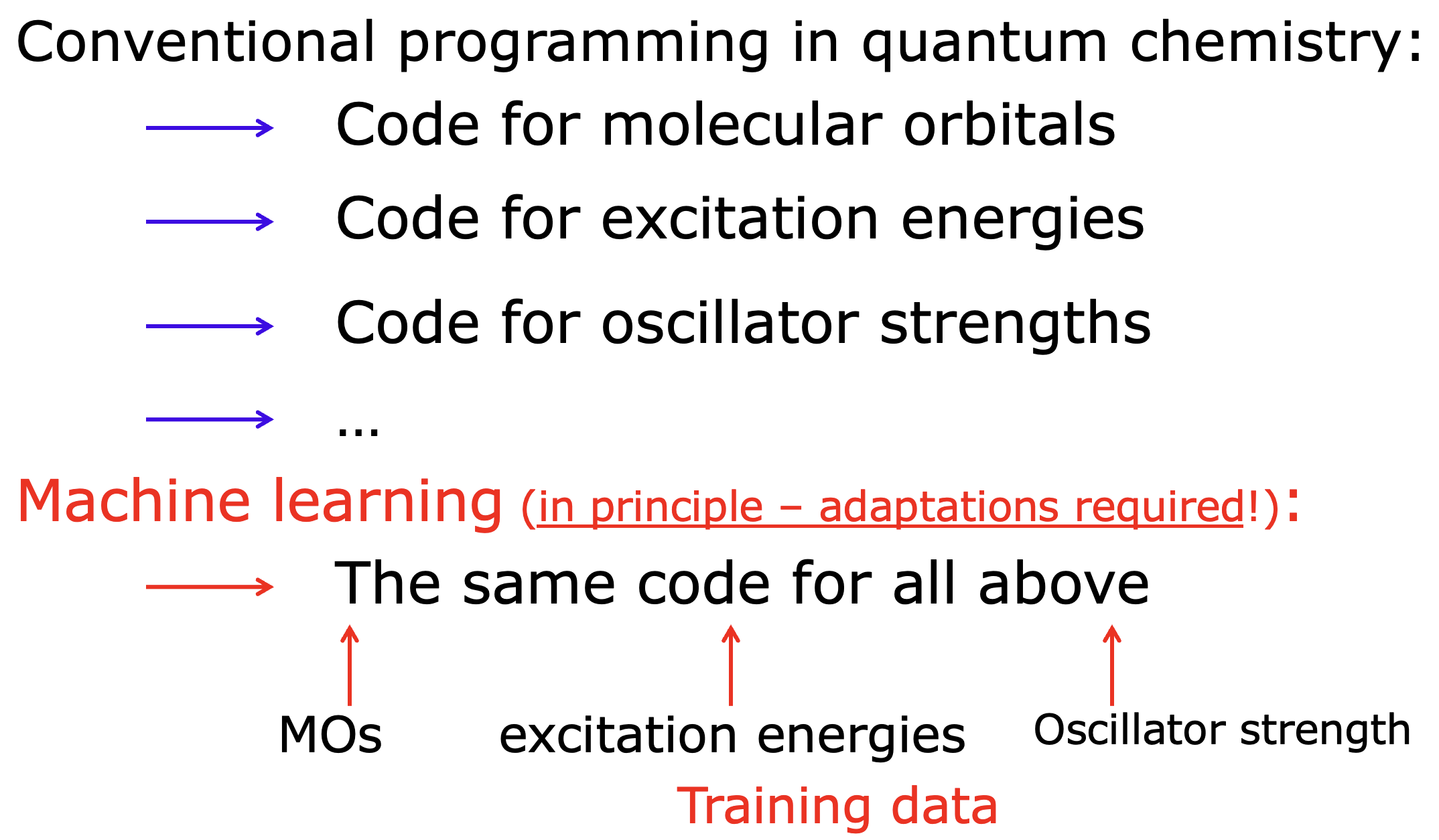
In ML-NEA, we create the KREG models to learn each property separately, i.e., we have twice as many models as excitations, because we learn both excitation energies and oscillator strengths. We also use kind of a pool-based active learning, where we keep sampling 50 more points from the Wigner distribution until the validation error in the ML models is decreasing less than by 10%:
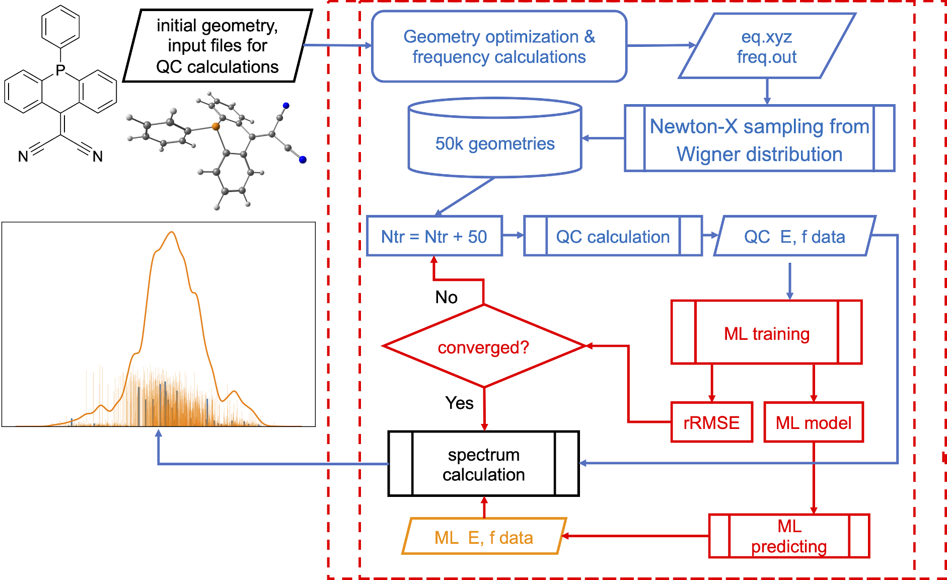
This allows us to obtain very precise spectra with confidence – in contrast to QM NEA we do not need to make subjective evaluation when stop sampling more points and what broadening factor to use. You can see it for yourself in the next exercise.
Example ML-spectra-3.
The following task is from our book chapter.
MLatom input file:
cross-section
Nexcitations=30
plotQCNEA
plotQCSPC
deltaQCNEA=0.05
These calculations require many data files (reference excitation energies at TDDFT level).
These data files are zipped. You should unzip them and upload all of them as auxiliary files to the cloud.
Create input file and submit the job in the File Manager.
Calculations can take more than 5 min. MLatom automatically determines the minimum required number of training points, in this case it needed 200 points for precise spectrum. In the output file you can find that it took 4 iterations to converge:
==========================================================================================
run ML-NEA iteratively for spectrum generation ( ML_train_iter ) started at Wed Dec  1 12:00:19 2021 CST
ML-NEA iteration 1: train_number = 50; RMSE_geom = 0.06717941145022376; rRMSE = 1.0

ML-NEA iteration 2: train_number = 100; RMSE_geom = 0.09043318436728051; rRMSE = 0.25713761026721255

ML-NEA iteration 3: train_number = 150; RMSE_geom = 0.06411060145373663; rRMSE = 0.410580813729204

ML-NEA iteration 4: train_number = 200; RMSE_geom = 0.0695737045717655; rRMSE = 0.07852252732055763

ML-NEA iteration ended after 4 iteration!
run ML-NEA iteratively for spectrum generation ( ML_train_iter ) finished at Wed Dec  1 12:08:01 2021 CST |||| total spent 462.02 sec
==========================================================================================
After the calculations finished, the spectra are plotted to plot.png file in the cross-section sub-directory. It should look like:
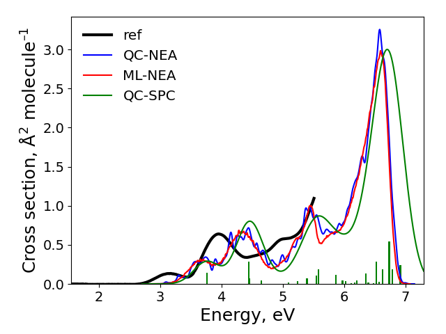
The final result: ‘ref’ is the experimental spectrum, QC-NEA – spectrum calculated with quantum chemical approach on 200 points in ensemble, ML-NEA – machine learning spectrum generated with 200 points in the training set and 50k points in ensemble, QC-SPC – spectrum generated with single-point convolution.
Compare obtained spectra and answer the following questions:
What are the problems with the QC-NEA spectrum?
What are the problems with the QC-SPC spectrum?
How to improve accuracy of the ML-NEA spectrum?
As you can see from this task, single-point convolution gives too simple of a spectrum and missing a finer band structure due to vibrations. Compared to QC-NEA spectrum, it is also shifted. QC-NEA spectrum has a problem of being too rough as evidently 250 points is not enough to provide a smooth spectrum. This leads to many spurious maxima. ML-NEA is the best but can be improved with more points further. However, this would not change the spectrum much. The best improvement would be by providing a better QM method to generate training data for ML.
You might have a question how to generate such a spectrum from scratch. You can do it if you install MLatom locally and have Gaussian program installed. We are planning to make ML-NEA also available on the XACS cloud computing in the future with alternative programs.
4.4. Emission spectra
Calculating emission spectra is similar to UV/vis with the major difference that we have to deal with the excited-state surface. E.g., if we use the single-point convolution then we need to optimize the geometry in the excited state (usually in the lowest excited state according to the Kasha’s rule). We applied it successfully to predict with AIQM1 that binding of fullerene with nanolassos quenches the fluorescence. However, on the cloud we can’t use the required MNDO program for this and, hence, such simulations are currently only possible locally (see instructions).
4.5. Two-photon absorption spectra
Two-photon absorption (TPA) is a fascinating property because it arises after two photons are absorbed simultaneously so that the electron is excited to a higher energy level than absorption of one photon of the same energy would make possible. Once the energy is pumped into molecule, it can release it back by emitting a photon of higher energy.
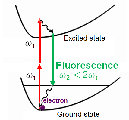
[Credit: By BP-Aegirsson - Own work, CC BY-SA 4.0]
This can be exploited in many applications such as upconverted laser, two-photon lithography, 3D printing, photodynamic therapy, and bioimaging.
Finding of molecules with strong TPA is therefore quite important. Unfortunately, the calculation of the TPA from first principles, i.e., with QM methods, is not an easy task and the accuracy of the affordable approaches is typically not high either. Hence, we developed a procedure to directly predict TPA with ML which is fast and comparable in accuracy to the DFT approaches. The calculations are quite simple as you just need to provide SMILES string of a molecule and information about the solvent and the range of wavelengths of photons to be absorbed (see the next task).
Example ML-spectra-4.
Taking an example from MLatom’s documentation, the input file to calculate the TPA of RHODAMINE 6G and RHODAMINE 123 molecules:
MLTPA
SMILESfile='
CCNC1=CC2=C(C=C1C)C(=C3C=C(C(=[NH+]CC)C=C3O2)C)C4=CC=CC=C4C(=O)OCC.[Cl-]
COC(=O)C1=CC=CC=C1C2=C3C=CC(=N)C=C3OC4=C2C=CC(=C4)N.Cl
'
auxfile='
600,850,55.4
600,600,33.9
'
After the calculations finish, the predicted TPA cross section values are saved in a folder named tpa[absolute time]. In the folder, there are two files for two molecules: tpa1.txt and tpa2.txt.
Analyze and plot the spectrum in tpa1.txt.
How long time did you take you to peform calculations?
The best answer to this exercise would tell which molecule out of the two has the strongest two-photon absorption and for the first molecule, where is the peak absorption.