7. Transition state search and analysis
The first-principles eludication of the reaction mechanism requires extensive simulations in time domain by also treating nuclei quantum mechanically (i.e., beyond Born–Oppenheimer approximation). However, in practice, this is rarely affordable and, hence, most of the simulations have to rely on a painstacking manual search of intermediates and transition states (TSs) to map the reaction profiles. There are new automatic tools reported each year and promissing to solve this problem, but so far practice shows that they all are not yet mature enough to deliver the routine simulations. However, it looks like we are on a brink of actually having such tools, potentially replacing the need for human experts doing these cumbersome tasks manually.
7.1. Slides
7.2. TS optimization
TS search is one of the most time-consuming and difficult tasks for a computational chemist which requries keen chemical understanding and intuition with calculations. The intuition can be obtained only via many trial-and-error attempts. Once TS found, you can calculate the reaction barrier (difference between the energies of the TS and reactants).
MLatom provides several ways to find transition states which you can find in the documentation. In the task below you can try out several of the simplest ones.
Example ML-TS-1.
Try to find a TS for the Diels–Alder reaction between ethylene and butadiene:

The most difficult part would be setting up a reasonable guess for the TS geometry used as an initial guess for TS optimization in MLatom. To simplify your life, we provide it.
An input file:
uaiqm
ts
xyzfile='16

C          0.48462430     -0.55755495      1.43729151
C          0.48462430     -0.55755495     -1.43729151
C         -0.27595797     -1.44977527      0.70359025
C         -0.27595797     -1.44977527     -0.70359025
C         -0.27595797      1.45086377      0.69299925
C         -0.27595797      1.45086377     -0.69299925
H          0.37292526     -0.50748993      2.51767690
H          1.44526264     -0.21636383      1.06867438
H          0.37292526     -0.50748993     -2.51767690
H          1.44526264     -0.21636383     -1.06867438
H         -1.05536225     -2.01444047      1.21328943
H         -1.05536225     -2.01444047     -1.21328943
H          0.51071931      1.96707995      1.23581344
H         -1.20625330      1.32768072      1.23591744
H          0.51071931      1.96707995     -1.23581344
H         -1.20625330      1.32768072     -1.23591744
'
optxyz=da_ts_opt.xyz
The TS should look something like this (depending on the level details may vary but it is a symmetric TS corresponding to the concerted mechanism):
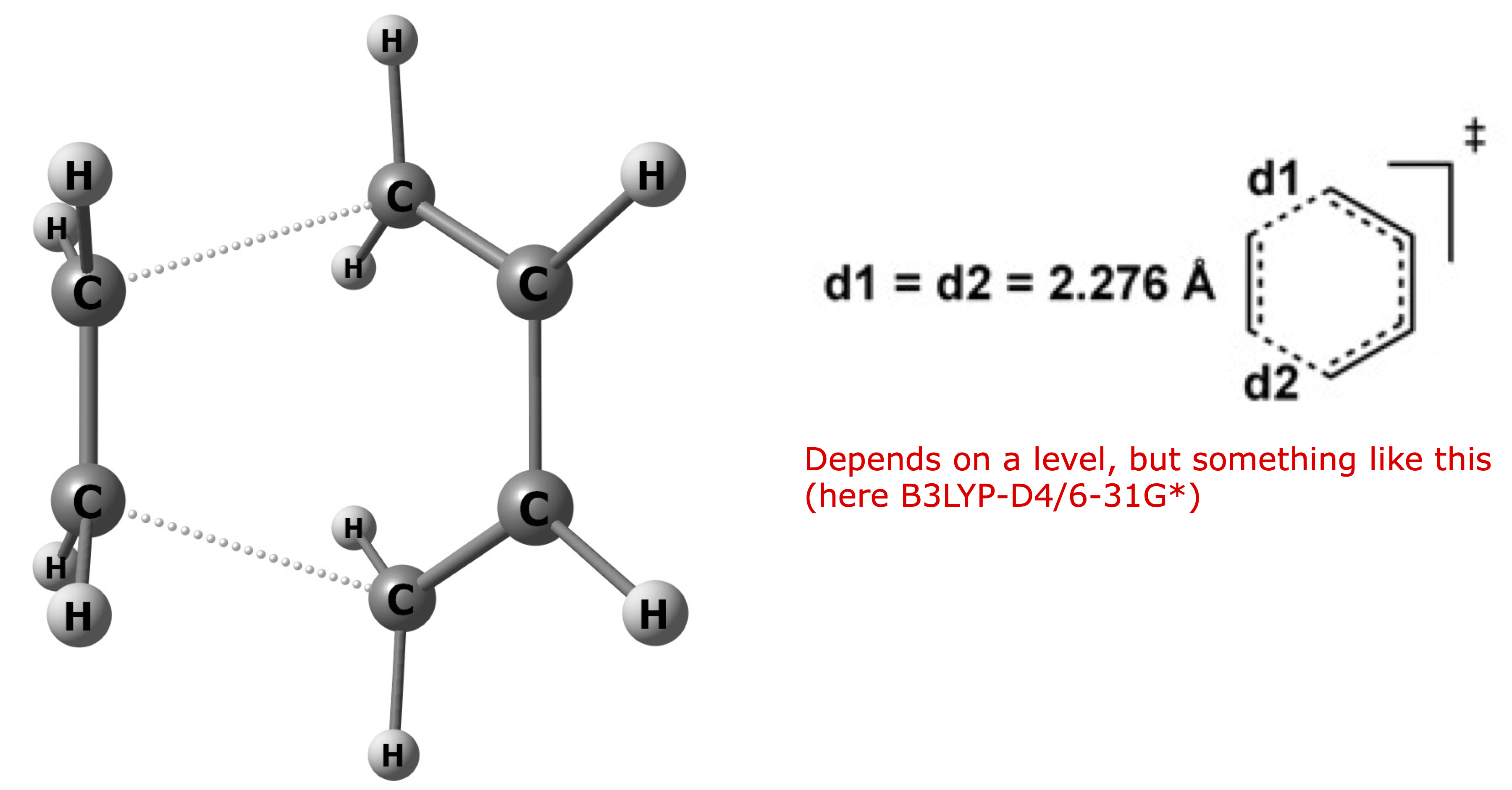
The optimized coordinates for your reference:
16

C             0.4984885582383          -0.5338087844381           1.4145928440825
C             0.4960692097735          -0.5384413336966          -1.4181301495364
C            -0.2896532359000          -1.4128506592682           0.7068921658160
C            -0.2905515192621          -1.4145888148315          -0.7051528877014
C            -0.2588083017453           1.4282744245852           0.6874347906976
C            -0.2574941435174           1.4288896351987          -0.6919434751381
H             0.3947104660660          -0.4397347928006           2.4878894665433
H             1.4467820702090          -0.2162549498538           1.0088131803715
H             0.3876593222716          -0.4479872886549          -2.4913060754311
H             1.4458716855847          -0.2184181276041          -1.0177581601047
H            -1.0783691986254          -1.9558675609816           1.2150705221731
H            -1.0799202791492          -1.9588818640283          -1.2105952858916
H             0.5409477501467           1.9087387905544           1.2339324532537
H            -1.1792980399036           1.2603193266422           1.2295776489298
H             0.5433702777959           1.9074275278623          -1.2394354082521
H            -1.1774768154298           1.2605820031641          -1.2339285873837
Importantly, the reaction kinetics is very sensitive to the errors in the barrier heights. Unfortunately, they are not obtained with high enough accuracy even with DFT. You may wonder how good are universal MLPs? UAIQM is quite good. Earlier, we benchmarked and found that ANI-1ccx is not even good for geometry optimizations while AIQM1 is better than semi-empirical methods for both geometry optimizations and energies but it is not even as good as DFT. This is not surprising given that no transition states were in the training data of either method. In addition, you may want to try a newer ANI-1xnr or other methods specifically trained on reaction data.
After the TSs located, it is important to confirm that the found structures actually correspond to the sought chemical transformation.
7.3. TS validation with normal modes
The first sanity check whether your optimized TS structure is the correct saddle point on the PES connecting reactants and products, is to perform the frequency calculations on it and confirm that it has only one imaginary (negative) frequency. This frequency corresponds to a normal mode which you can visualize and check whether this vibration corresonds to the sought reaction coordinate.
In addition, frequency calculations will give you thermochemical properties which you can use to calculate the Gibbs free energy of activation.
Example ML-TS-2.
For the structure(s) you found in the previous task, calculate frequencies:
freq
uaiqm
xyzfile='16

C             0.4984885582383          -0.5338087844381           1.4145928440825
C             0.4960692097735          -0.5384413336966          -1.4181301495364
C            -0.2896532359000          -1.4128506592682           0.7068921658160
C            -0.2905515192621          -1.4145888148315          -0.7051528877014
C            -0.2588083017453           1.4282744245852           0.6874347906976
C            -0.2574941435174           1.4288896351987          -0.6919434751381
H             0.3947104660660          -0.4397347928006           2.4878894665433
H             1.4467820702090          -0.2162549498538           1.0088131803715
H             0.3876593222716          -0.4479872886549          -2.4913060754311
H             1.4458716855847          -0.2184181276041          -1.0177581601047
H            -1.0783691986254          -1.9558675609816           1.2150705221731
H            -1.0799202791492          -1.9588818640283          -1.2105952858916
H             0.5409477501467           1.9087387905544           1.2339324532537
H            -1.1792980399036           1.2603193266422           1.2295776489298
H             0.5433702777959           1.9074275278623          -1.2394354082521
H            -1.1774768154298           1.2605820031641          -1.2339285873837
'
If you done everything properly, the normal mode corresponding to the reaction coordinate would look like:
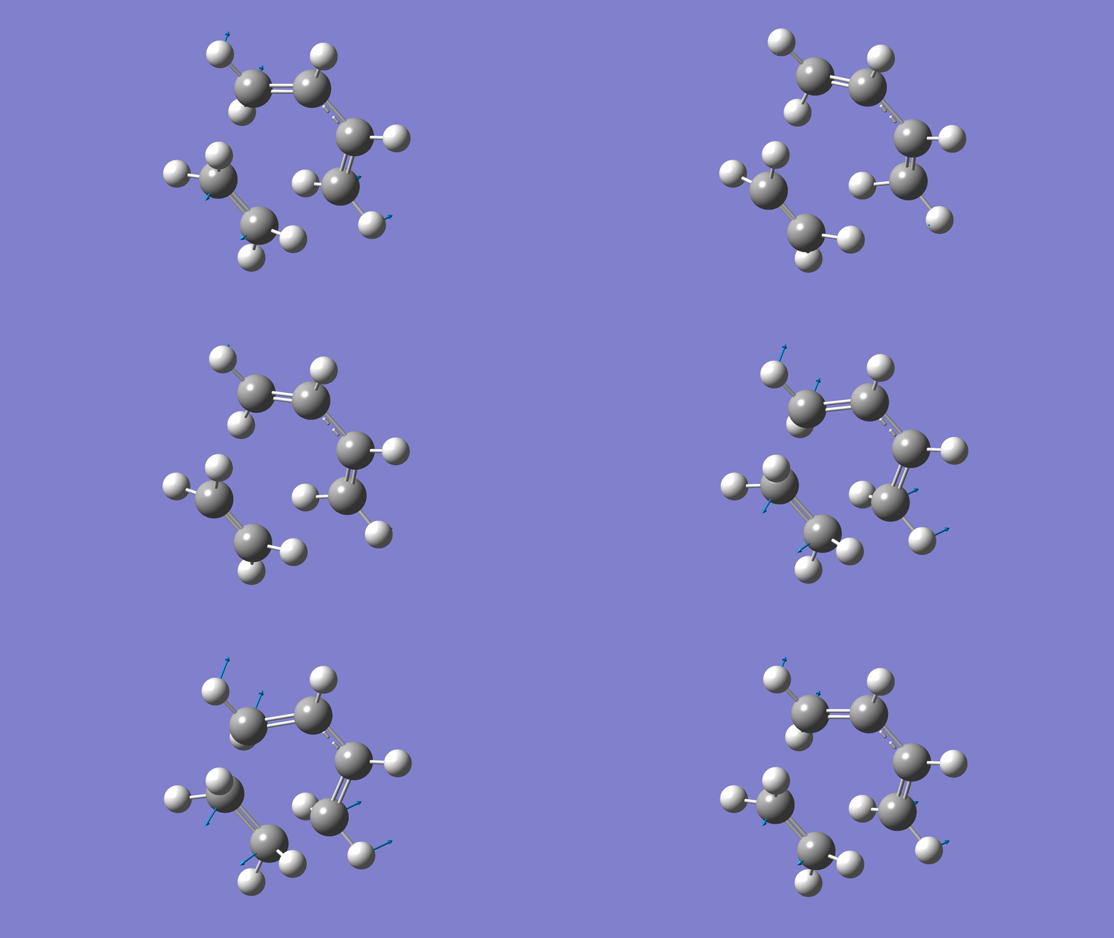
[Credit: taken from MLatom’s documentation]
Note
If you wonder how to make such an animation: we used Gaussian to run frequency calculations with our model, and the Gaussian output can be visualized with Gaussview or ChemCraft. We can’t provide Gaussian on the cloud computing though. We will provide a work-around soon – please subscribe to our updates on WeChat!
The output will contain one negative frequency:
Mode     Frequencies     Reduced masses     Force Constants
            (cm^-1)            (AMU)           (mDyne/A)
    1       -599.9203          8.3844            -1.7779
    2         55.2239          5.8098             0.0104
    3        137.6350          2.0276             0.0226
    4        259.0093          2.8785             0.1138
    5        364.0193          3.9539             0.3087
    6        375.8171          2.3977             0.1995
    ...
7.4. Intrinsic reaction coordinate (IRC)
The more rigorous check for the correctness of the optimized TS structure is following intrinsic reaction coordinate (IRC). IRC follows the minimum-energy path from TS to reactants and products and you can analyze the structures along this path as well the energy profile. Performing IRC is more rigorous than simply checking the normal mode corresponding to the reaction coordinate.
If you have a Gaussian program and installed MLatom locally, the input file to MLatom is very simple:
# first of all, choose the method!
IRC
xyzfile=... # file with the optimized TS structure
Then you can check whether the IRC leads to the reactants and products you expect. You can also check the energy profile along the reaction coordinate which may look like this (details will vary depending your level):
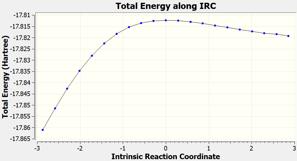
[Credit: taken from MLatom’s documentation]
7.5. TS analysis via downhill dynamics
The problem with IRC that it goes along the minimum-energy path while real reactions never exactly stick to it. The molecules always are in complex dynamical motions and hence it is more appropriate to perform dynamics to find reaction events. Unfortunately, reaction time scales are typically too long to be directly assessed in MD. The compromise is to find TS and start MD downhill from this TS to products. Also, typically, we need to sample geometries around TS to reflect that the reaction never exactly passes through the TS. A powerful and common tool for this is quasi-classical trajectories which we already encountered before. A special consideration has to be taken that during the sampling of initial conditions, they are sampled from the normal modes orthogonal to the reaction coordinate. This is done automatically in MLatom. Since the trajectories are very slow, it is better to use active learning procedures to generate a good ML potential and accelerate such downhill MD exploration. Also, you would need to run thousands of trajectories in both forward and backward directions to properly analyze the distribution of the reaction outcomes, particularly for the reactions with post-TS bifurcation (very interesting class of reactions where you can observe formation of several different products from the same TS!).
You can try yourself to run downhill MD from the TS:
Example ML-TS-3.
Run several quasi-classical trajectories for the Diels–Alder reaction starting from the TS.
Analyze where this dynamics leads. Is it consistent with the previous analysis with normal modes and IRC?
MD
MLmodelType=ANI
MLmodelIn=da_energy_ani.npz
initConditions=harmonic-quantum-boltzmann
normalModeFile=da_eqmol.json
initTemperature=300
trun=150
dt=0.5
For this dynamics, you need:
da_eqmol.json- file with frequencies and normal modes: (you can generate such files when you performfreqcalculations with MLatom, they will be stored infreq1.json).da_energy_ani.npz- ANI model pretrained on B3LYP/6-31G* data for you. You can use your own level of theory but this dynamics might be quite slow while ML model is much faster.
If you use the same initial conditions but flip the sign in velocities, you can get the set of forward and backward trajectories which you can later put together in one trajectory. If this trajectories goes from reactants to products (or vice versae), it is reactive but some small fraction of trajectories will be non-reactive (i.e., starting and ending with reactants or products).
When you run many such dynamics you can obtain beautiful reaction trajectories like we obtained:
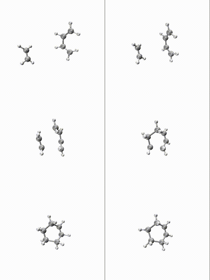
For larger reactions, you can even find some roaming like we did for the Diels–Alder reaction of fullerene with 2,3-dimethyl-1,3-butadiene:
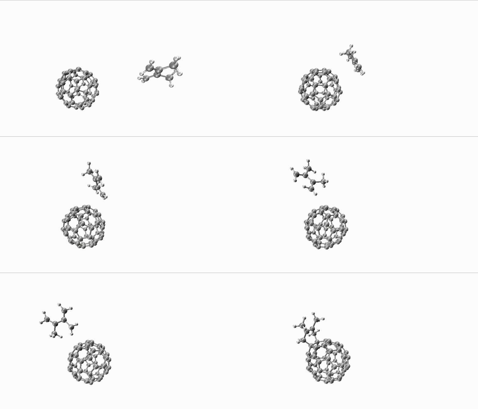
You can only obtain such insights with thousands of long trajectories which are much faster with MLPs.
7.6. Quasiclassical trajectories analysis on the bifurcating pericyclic reaction
If you ever wondered how to get the computation of the beautiful reaction mechanisms, below are instructions from MLatom’s documentation prepared by Yuxinxin Chen.
In this section, we will reproduce the quasiclassical trajectories for bifurcating pericyclic reaction reported in JACS (2017) 139, 8251, where the human experts manually chosen the B3LYP-D3/6-31G* level of theory and got the distribution of the products with the resulting 117 reactive trajectories. With the UAIQM models, we can quickly shoot 1000 trajectories and get 867 reactive ones, while the energy profile is more accurate than B3LYP which is known for low reliability on energy prediction.
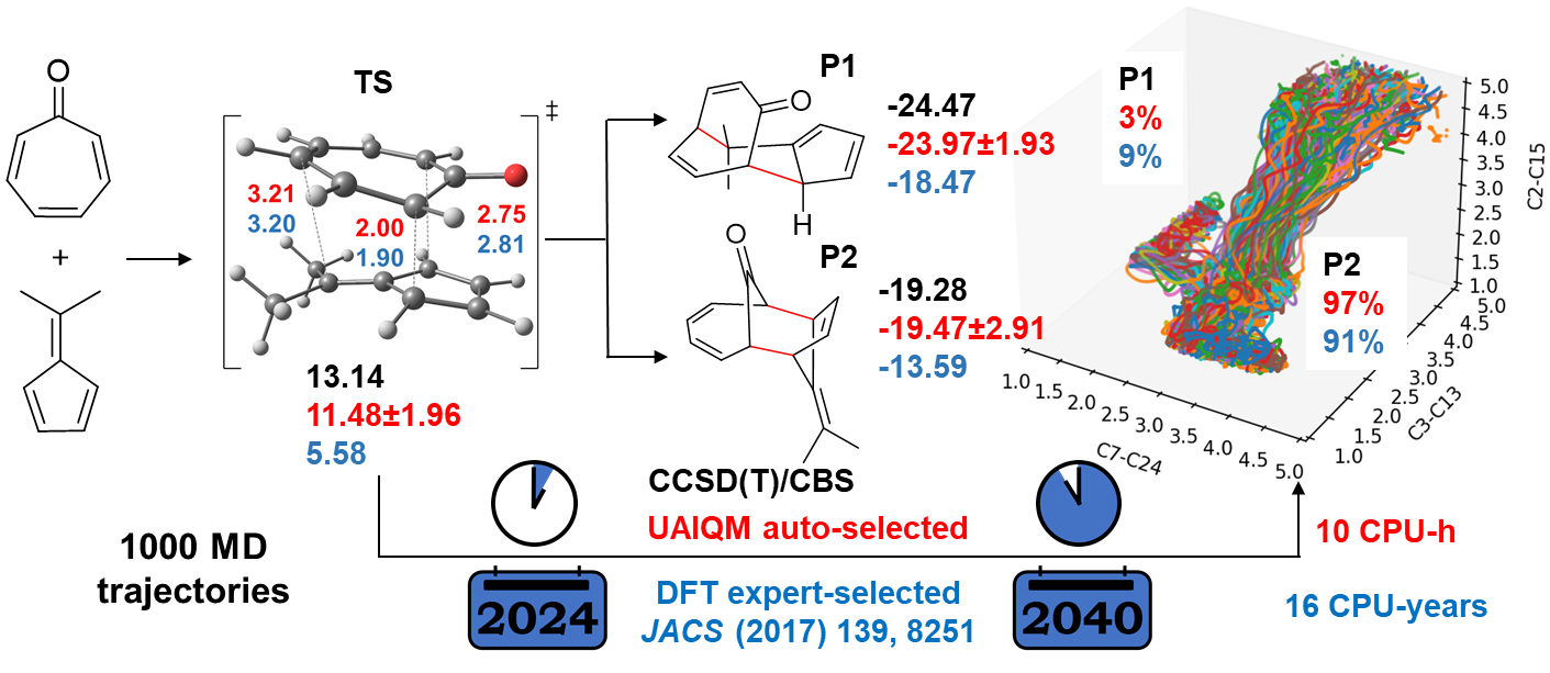
Below we provide instructions on the procedure to propagate one trajectory in less than one minute with our UAIQM models. Time budget is reduced to 0.1 s for UAIQM method. The same setting for quasi-classical MD will be used as that in the original paper, i.e. 500 fs long trajectory with 1 fs time step starting from region near ambimodal transition state. Initial transition state file can be downloaded: TS1.xyz.
import mlatom as ml

# load initial transitiona state
init_ts1 = ml.data.molecule.from_xyz_file('TS1.xyz')

# choose optimal UAIQM method
uaiqm_optimal = ml.models.uaiqm(method='uaiqm_optimal', verbose=False)
uaiqm_optimal.select_optimal(
    molecule=init_ts1,
    nCPUs=1,
    time_budget='0.1s'
)

# optimize geometry and get frequencies
geomopt = ml.optimize_geometry(
    model=uaiqm_optimal,
    initial_molecule=init_ts1,
    ts=True,
    program='geometric'
)
optmol_ts1 = geomopt.optimized_molecule
ml.freq(model=uaiqm_optimal, molecule=optmol_ts1)

# get initial conditions
for ifreq in range(len(optmol_ts1.frequencies)):
    if optmol_ts1.frequencies[ifreq] > 0 and optmol_ts1.frequencies[ifreq] < 100:
        optmol_ts1.frequencies[ifreq] = 100

init_cond_db = ml.generate_initial_conditions(molecule=optmol_ts1,
                                            generation_method='harmonic-quantum-boltzmann',
                                            number_of_initial_conditions=1000,
                                            initial_temperature=298,
                                            use_hessian=False)
# dump forward initial conditions
init_cond_db.dump(f'TS1_incond_298.json',format='json')

# Reverse the velocities to get the backward trajectories
re_init_cond_db = init_cond_db.copy()
for mol in re_init_cond_db:
    for atom in mol:
        atom.xyz_velocities = -atom.xyz_velocities
# dump backward initial conditions
re_init_cond_db.dump(f're_TS1_incond_298.json',format='json')

# propagate one forward trajectory
init_mol = init_cond_db[0]
dyn = ml.md(model=uaiqm_optimal,
            molecule_with_initial_conditions = init_mol,
            ensemble='NVE',
            time_step=1,
            maximum_propagation_time=500,
            )
traj = dyn.molecular_trajectory
traj.dump(filename=f'forward_temp298_mol0', format='plain_text')

# propagate backward trajectory
re_init_mol = re_init_cond_db[0]
dyn = ml.md(model=uaiqm_optimal,
            molecule_with_initial_conditions = re_init_mol,
            ensemble='NVE',
            time_step=1,
            maximum_propagation_time=500,
            )
traj = dyn.molecular_trajectory
traj.dump(filename=f'backward_temp298_mol0', format='plain_text')

# check reactive trajectories
import numpy as np
def get_bond_data(traj_xyz, bonds):
    nmol = len(traj_xyz)
    data = np.zeros((nmol, len(bonds)))
    for ii in range(nmol):
        mol = traj_xyz[ii]
        bl_list = []
        for bond in bonds:
            bl = mol.internuclear_distance(bond[0], bond[1])
            bl_list.append(bl)
        data[ii] = bl_list
    return data

def check_reactive(traj_bond_data):
    P1 = False # C2-C15 C7-C24
    P2 = False # C2-C15 C3-C13
    for ii in range(traj_bond_data.shape[0]):
        bond_data = traj_bond_data[ii]
        if bond_data[0] <= 1.6 and bond_data[1] <= 1.6:
            P2 = True
        if bond_data[0] <= 1.6 and bond_data[2] <= 1.6:
            P1 = True

    return P1, P2

bonds = [(1,14),(2,12),(6,23)]
traj_forward = ml.data.molecular_database.from_xyz_file(f'forward_temp298_mol0.xyz')
traj_backward = ml.data.molecular_database.from_xyz_file(f'backward_temp298_mol0.xyz')
traj = ml.data.molecular_database()
traj_forward.molecules.reverse()
traj.molecules = traj_forward.molecules + traj_backward.molecules
P1, P2 = check_reactive(get_bond_data(traj, bonds=bonds))
print(f'P1 in trajectory: {P1}\n')
print(f'P2 in trajectory: {P2}\n')