9. Surface-hopping nonadiabatic dynamics
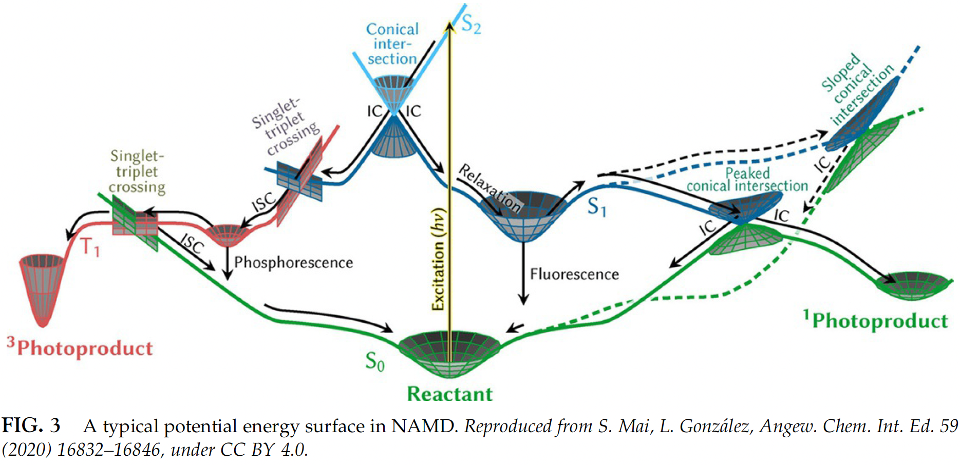
Many processes, i.e., photophysics and photochemistry but also many reactions, occur not just on a ground-state PES but involve other electronic states:

Simulating their dynamics properly is even more complicated. One of the most popular approaches is the so-called surface-hopping nonadiabatic dynamics where many trajectories are propagated starting from different states. In each trajectory, the molecule is allowed to hop from one electronic surface to another and then we can count how many trajectories at a given time stay on each surface (the percentage is called population). This is very computationally intensive task and, hence, ML is also eagerly awaited solution which is still far from trivial to use in nonadiabatic simulations. MLatom can also perform such simulations but currently only in Python. The results with AIQM1 which does not need any training are often quite good too.
The tutorial below is adapted from MLatom’s documentation prepared together with Lina Zhang.
In this tutorial we show how to perform nonadiabatic molecular dynamics (NAMD) with MLatom (and its interfaces to Newton-X whenever required). The simulations are only possible through the Python API. MLatom currently only supports NAC-free Landau–Zener–Belyev–Lebedev (LZBL) surface hopping.
Here we show two examples of how to propagate dynamics with:
the universal AIQM1 method (ML-improved semi-empirical QM approach faster than DFT)
See our paper for more details (please also cite it if you use this feature):
Lina Zhang, Sebastian Pios, Mikołaj Martyka, Fuchun Ge, Yi-Fan Hou, Yuxinxin Chen, Joanna Jankowska, Lipeng Chen, Mario Barbatti, Pavlo O. Dral. MLatom software ecosystem for surface hopping dynamics in Python with quantum mechanical and machine learning methods. J. Chem. Theory Comput. 2024, 20, 5043–5057. DOI: 10.1021/acs.jctc.4c00468. Preprint on arXiv: https://arxiv.org/abs/2404.06189.
9.1. Slides
9.2. Machine learning
In this tutorial, we show a more advanced example of running surface-hopping MD with ML models. Please see a separate tutorial on machine learning potentials in general and later we will provide tutorials on how to train MLPs specifically for excited states.
You can download the Jupyter notebook with the required initial conditions and ML models from this paper.
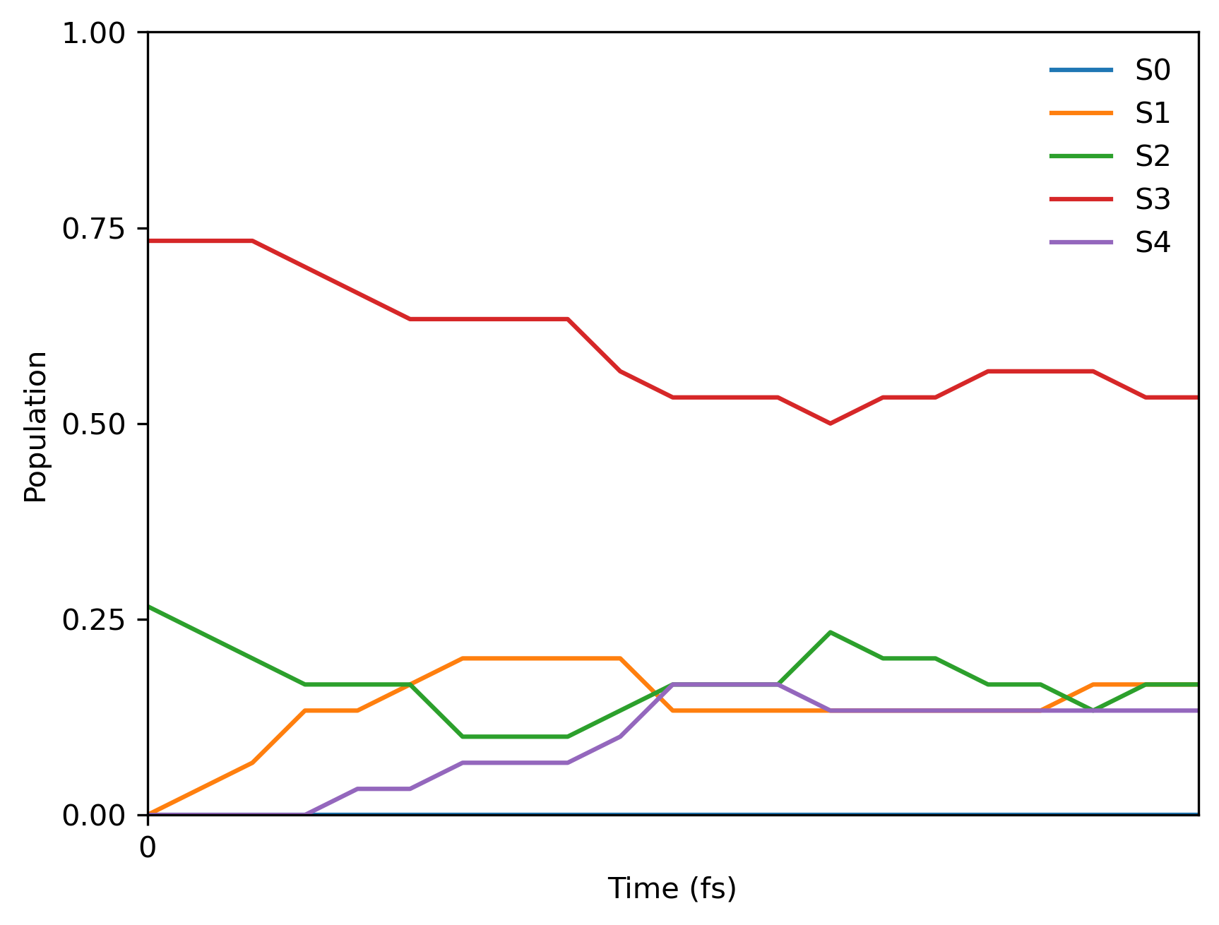
The tutorial calculations are very fast and you should be able to get the final population plot for 5 fs with 0.25 fs time step from 30 trajectories within a minute. Here is the Jupyter notebook code snippet:
import mlatom as ml
import os
import numpy as np

# Read initial conditions
init_cond_db = ml.data.molecular_database.load(filename='materials/init_cond_db_for_pyrazine.json', format='json')

# We need to create a class that accepts the specific arguments shown below and saves the calculated electronic state properties in the molecule object
class mlmodels():
    def __init__(self, nstates = 5):
        folder_with_models = 'materials/lz_models'
        self.models = [None for istate in range(nstates)]
        for istate in range(nstates):
            self.models[istate] = [ml.models.ani(model_file=f'{folder_with_models}/ensemble{ii+1}s{istate}.pt') for ii in range(2)]
            for ii in range(2): self.models[istate][ii].nthreads = 1

    def predict(self,
            molecule=None,
            nstates=5,
            current_state=0,
            calculate_energy=True,
            calculate_energy_gradients=True):

        molecule.electronic_states = [molecule.copy() for ii in range(nstates)]

        for istate in range(nstates):
            moltmp = molecule.electronic_states[istate]
            moltmpens = [moltmp.copy() for ii in range(2)]
            for ii in range(2):
                self.models[istate][ii].predict(molecule=moltmpens[ii], calculate_energy = True, calculate_energy_gradients = True)
            moltmp.energy = np.mean([moltmpens[ii].energy for ii in range(2)])
            moltmp.energy_gradients = np.mean([moltmpens[ii].energy_gradients for ii in range(2)], axis=0)

        molecule.energy = molecule.electronic_states[current_state].energy
        molecule.energy_gradients = molecule.electronic_states[current_state].energy_gradients

models = mlmodels()

# Arguments for running NAMD trajectories
timemax = 5 # fs
namd_kwargs = {
            'model': models,
            'time_step': 0.25, # fs
            'maximum_propagation_time': timemax,
            'dump_trajectory_interval': None,
            'hopping_algorithm': 'LZBL',
            'nstates': 5,
            'random_seed': 1, # making sure that the hopping probabilities are the same (should not be used in actual calculations!)
            'rescale_velocity_direction': 'along velocities',
            'reduce_kinetic_energy': False,
            }

# Run 30 trajectories
dyns = ml.simulations.run_in_parallel(molecular_database=init_cond_db[:30], task=ml.namd.surface_hopping_md, task_kwargs=namd_kwargs)
trajs = [d.molecular_trajectory for d in dyns]
ml.namd.analyze_trajs(trajectories=trajs, maximum_propagation_time=timemax)

# Dump the trajectories
for itraj in range(len(trajs)):
    trajs[itraj].dump(filename=f'traj{itraj+1}.json', format='json')

# Prepare the population plot
ml.namd.plot_population(trajectories=trajs, time_step=0.25,
                        max_propagation_time=timemax, nstates=5, filename=f'pop.png')
Since we used the fixed random seed, you should get the following final population:

9.3. Setup for calculations on your computer with AIQM1
Depending on the electron structure method or machine learning model, you might need to install the development version of MLatom and external programs such as MNDO (required for AIQM1 and semi-empirical QM), COLUMBUS (required for CASSCF), Turbomole (required for ADC(2)), or TorchANI (required for AIQM1 and ANI potentials). dftd4 is also required for AIQM1.
9.4. AIQM1
This tutorial consists of two parts:
single-point calculations to better understand how to use MLatom for excited-state calculations
surface-hopping dynamics building upon the previous example.
9.4.1. Single-point excited-state calculations
Please download the tutorial files (sp_aiqm1.zip).
To start, we provide the initial geometry for \(\text{CNH}_4^+\) in the cnh4+.xyz file, with coordinates in Angstrom, which looks like this:
6
symmetry c1
N        0.051443000     -0.125748000      0.596619000
C        0.067113000     -0.025698000     -0.683445000
H        0.002169000      0.695516000      1.199263000
H        0.087711000     -1.030762000      1.065358000
H        0.027120000      0.954772000     -1.143351000
H        0.120118000     -0.922908000     -1.288953000
Then we can use this geometry to calculate the excited-state properties at the AIQM1/CIS level (in the comments also for AIQM1/MRCI):
#!/usr/bin/env python
# coding: utf-8

import mlatom as ml

# get the molecule object
mol = ml.data.molecule()
mol.read_from_xyz_file('cnh4+.xyz')
mol.charge = 1

# define the method
aiqm1 = ml.models.methods(method='AIQM1')
# To run AIQM1/MRCI calculations, you can uncomment the following line and make sure that mndokw file is available (see below)
#aiqm1 = ml.models.methods(method='AIQM1',qm_program_kwargs={'read_keywords_from_file':'mndokw'})

# calculate electronic state properties
aiqm1.predict(molecule=mol,
                nstates=3, # Number of electronic states to calculate
                current_state=2, # Requests calculating properties for the S2 electronic state (the third one or second excited)
                calculate_energy=True,
                calculate_energy_gradients=[True, True, True], # requests calculating gradients for all three states
                #calculate_energy_gradients=True # requests calculating gradients only for the current state for many methods (but not for AIQM1 yet)
                calculate_nacv=False, # calculate nonadiabatic coupling vectors
                read_density_matrix=False)

# show the energy and gradients of each state
for i in range(len(mol.electronic_states)):
    print(f'Energy of state {i}, {mol.electronic_states[i].energy}')
    print(f'Energy gradients of state {i}')
    print(mol.electronic_states[i].energy_gradients)

# or alternatively:
print('Electronic state energies:', mol.state_energies)
print('Energy gradients in all electronic states')
print(mol.state_gradients)

# save the molecule object in file
mol.dump(filename="mol.json", format="json")
The output produced by the above Python script will look like this:
Energy of state 0, -94.87746605828193
Energy gradients of state 0
[[-2.20979325e-05 -3.09923481e-05  4.19648750e-04]
[ 1.84361461e-05  7.32504232e-05 -9.31292919e-04]
[-2.19042984e-04  4.91462433e-03 -8.93827657e-04]
[ 2.61506161e-04 -4.71725762e-03 -1.64437563e-03]
[ 1.19805843e-04 -2.90049761e-03  1.30834139e-03]
[-1.58607238e-04  2.66087287e-03  1.74150332e-03]]
Energy of state 1, -94.63515481241645
Energy gradients of state 1
[[ 5.04737245e-04  3.19599783e-03 -4.08726944e-02]
[ 4.00318642e-04  2.59615245e-03 -3.32555938e-02]
[ 2.10040873e-04  2.67707897e-05 -1.31297761e-02]
[ 1.06425061e-04  2.01394042e-03 -1.29785531e-02]
[-1.28339570e-04 -1.37049107e-02  4.93587653e-02]
[-1.09318226e-03  5.87204910e-03  5.08778502e-02]]
Energy of state 2, -94.58438542616139
Energy gradients of state 2
[[-3.22384930e-04 -1.95587619e-03  2.50398870e-02]
[ 1.58487817e-03  1.00715972e-02 -1.28916150e-01]
[-9.11050390e-06  3.73598849e-03 -1.03835407e-02]
[ 2.78260000e-04 -2.07710696e-03 -1.08367181e-02]
[ 2.43944556e-03 -6.96100621e-02  5.75290677e-02]
[-3.97108828e-03  5.98354594e-02  6.75674517e-02]]

Electronic state energies: [-94.87746606 -94.63515481 -94.58438543]
Energy gradients in all electronic states
[[[-2.20979325e-05 -3.09923481e-05  4.19648750e-04]
...
All results of the calculations will be dumped into mol.json which you can inspect to get a better idea how the data are stored in MLatom and how to access different properties through its Python API.
If you used AIQM1/MRCI, you would need to select active space and make other adjustments to the keywords passed to the MNDO program (see its documentation). In our case, you would need to use mndokw file which looks like this:
jop=-2 +
iop=-22 immdp=-1 igeom=1 iform=1 nsav15=3 +
icuts=-1 icutg=-1 kitscf=9999 iscf=9 iplscf=9 +
iprint=-1 kprint=-5 lprint=-2 mprint=0 jprint=-1 +
kharge=1 imult=0 nprint=-1 +
kci=5 movo=-1 ici1=2 ici2=1 jci1=1 jci2=1 nciref=0 +
iroot=3 iuvcd=2 +
ncisym=-1 ioutci=3 ipubo=1 +
ncigrd=3 icross=1
The output would be then:
Energy of state 0, -94.88480497779682
Energy gradients of state 0
[[ 1.34242995e-04  9.67083232e-04 -1.23502153e-02]
[-1.78362286e-04 -1.17842971e-03  1.50824778e-02]
[-9.10435874e-05  2.63194636e-03 -2.00336109e-03]
[ 1.56325835e-04 -2.28966888e-03 -2.38851941e-03]
[ 3.31705685e-05 -9.16708517e-04  7.62840787e-04]
[-5.43335121e-05  7.85777537e-04  8.96776412e-04]]
Energy of state 1, -94.63484529385708
Energy gradients of state 1
[[ 0.00050423  0.00321188 -0.04107714]
[ 0.00044946  0.00290478 -0.0372039 ]
[ 0.00017054  0.00049241 -0.01193939]
[ 0.00012002  0.001369   -0.01187431]
[-0.00012679 -0.01405619  0.0502662 ]
[-0.00111746  0.00607812  0.05182854]]
Energy of state 2, -94.56976745482731
Energy gradients of state 2
[[ 6.21429387e-03  3.96821088e-02 -5.07668904e-01]
[-6.24036735e-03 -3.98880933e-02  5.10344195e-01]
[-9.20936201e-05  2.29106816e-03 -1.36149279e-03]
[ 1.28184773e-04 -2.05330005e-03 -1.70182967e-03]
[ 9.81727653e-05 -2.05300286e-03  3.51054010e-05]
[-1.08190451e-04  2.02121919e-03  3.52925482e-04]]
9.4.2. Dynamics
Here we extend above example to show row to use the same method as before (AIQM1/MRCI) in propagating LZBL surface-hopping dynamics. Please download the tutorial files (namd_aiqm1.zip).
The script below does all the steps from start to finish:
optimizes geometry
runs frequency calculations
samples initial conditions from the Wigner distribution using Newton-X’s routines. Example can be extended to supports filtering by excitation energy window (refer to the manual for more details)
propagates multiple trajectories in parallel (here 16 trajectories for 5 fs with 0.1 fs time step)
saves trajectories in the h5md format
analyzes results by generating the population plots.
Here is the script:
import mlatom as ml

# Load the initial geometry of a molecule
mol = ml.data.molecule()
mol.charge=1
mol.read_from_xyz_file('cnh4+.xyz')

# Define methods
# .. for NAMD
aiqm1 = ml.models.methods(method='AIQM1',
                        qm_program_kwargs={'save_files_in_current_directory': True,
                                            'read_keywords_from_file':'../materials/mndokw'})
# .. for optimization, frequencies and normal mode calculations
method_optfreq = ml.models.methods(method='B3LYP/Def2SVP', program='pyscf')

# Optimize geometry
geomopt = ml.simulations.optimize_geometry(model=method_optfreq,
                                        initial_molecule=mol)
eqmol = geomopt.optimized_molecule
eqmol.write_file_with_xyz_coordinates('eq.xyz')

# Get frequencies
ml.simulations.freq(model=method_optfreq,
                    molecule=eqmol)
eqmol.dump(filename='eqmol.json', format='json')

# Get initial conditions
init_cond_db = ml.generate_initial_conditions(molecule=eqmol,
                                    generation_method='wigner',
                                    number_of_initial_conditions=16,
                                    initial_temperature=0,
                                    random_seed=1) # To ensure we always get the same initial conditions (should not be used in actual calculations)
init_cond_db.dump('test.json','json')

# Propagate multiple LZBL surface-hopping trajectories in parallel
# .. setup dynamics calculations
namd_kwargs = {
            'model': aiqm1,
            'time_step': 0.25,
            'maximum_propagation_time': 5,
            'hopping_algorithm': 'LZBL',
            'nstates': 3,
            'initial_state': 2, # Numbering of states starts from 0!
            'random_seed': 1 # To ensure we always get the same initial conditions (should not be used in actual calculations)
            }

# .. run trajectories in parallel
dyns = ml.simulations.run_in_parallel(molecular_database=init_cond_db,
                                      task=ml.namd.surface_hopping_md,
                                      task_kwargs=namd_kwargs,
                                      create_and_keep_temp_directories=True)
trajs = [d.molecular_trajectory for d in dyns]

# Dump the trajectories
itraj=0
for traj in trajs:
    itraj+=1
    traj.dump(filename=f"traj{itraj}.h5",format='h5md')

# Analyze the result of trajectories and make the population plot
ml.namd.analyze_trajs(trajectories=trajs, maximum_propagation_time=5)
ml.namd.plot_population(trajectories=trajs, time_step=0.25,
                        max_propagation_time=5, nstates=3, filename=f'pop.png', pop_filename='pop.txt')
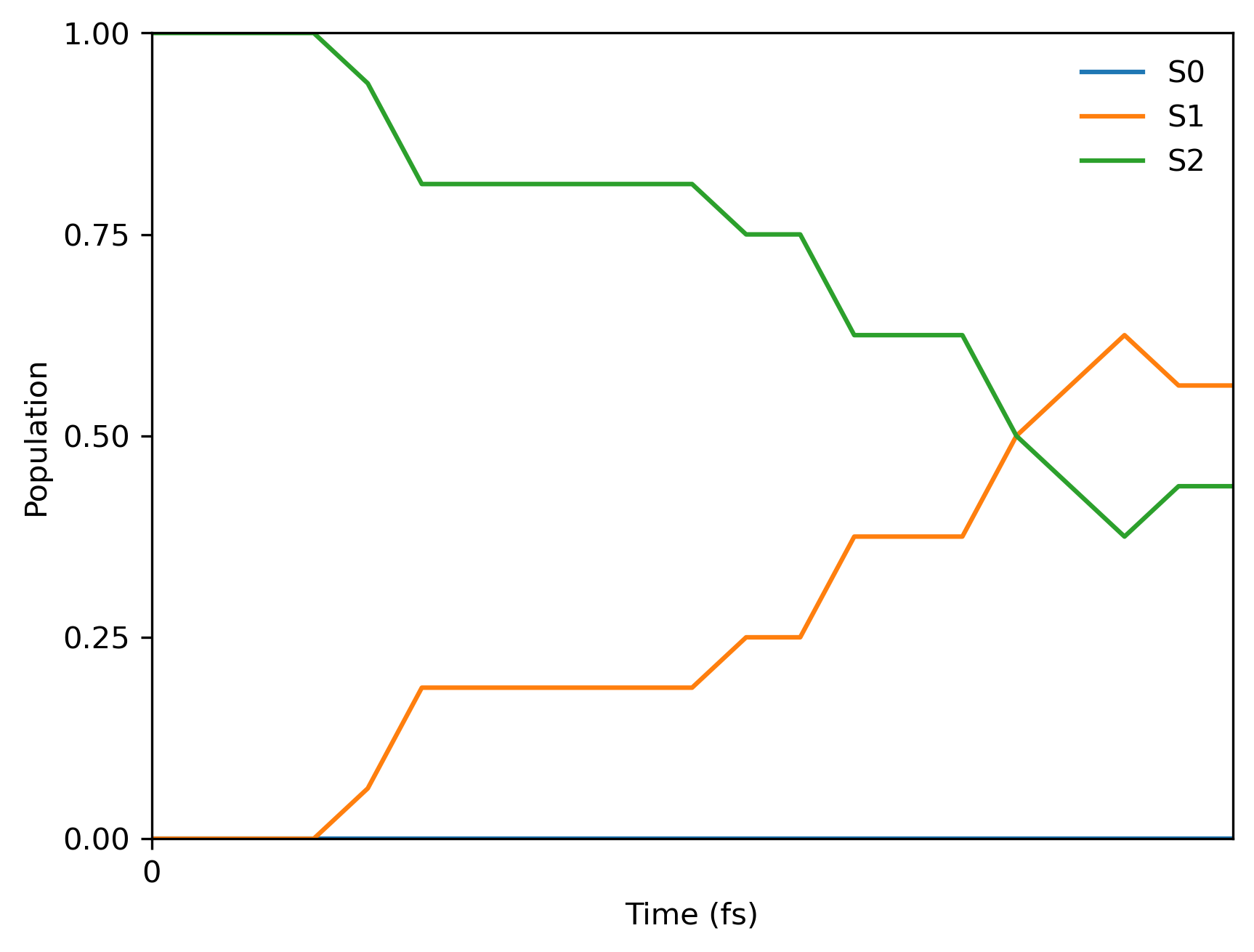
And here is the final population plot (your plot will be different because of the random seed in initial conditions and hoppings):

You will also get the text file with populations pop.txt which should look like:
0.000 0.0 0.0 1.0
0.250 0.0 0.0 1.0
0.500 0.0 0.0 1.0
0.750 0.0 0.0 1.0
...
Download the full file cnh4+_aiqm1cis_lznamd_population.txt.